
Integrated Deployment is an innovative technique for the direct deployment of data science. It allows the data scientist to model both data science creation and production within the same environment by capturing the parts of the process that are needed for deployment. One subset of integrated deployment, for example, is the deployment of machine learning models.
When building machine learning models it is notorious that one of the biggest problems of the deployment step is the safe capturing of the models and all the related data transformations for the production environment. Mistakes made in transferring the right transformations with the right parameters invalidate the whole deployment procedure and therefore also the whole model training behind it.
The innovative character of the integrated deployment technique changes the “moving into production” into a faithful “capturing” of the relevant data computations directly from the model training.
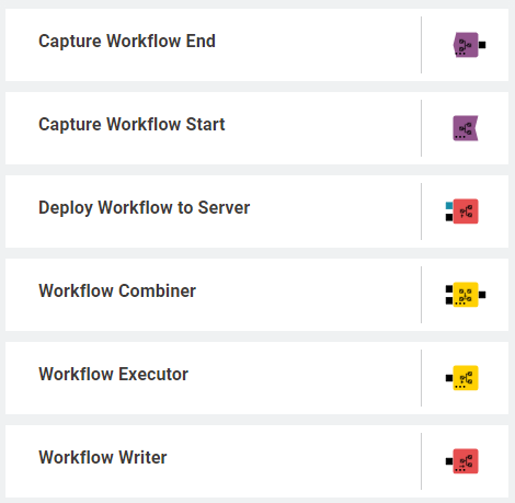
Like many other free and open source KNIME Extensions, the KNIME Integrated Deployment extension comes as a collection of nodes (Fig. 1), as usual available on the KNIME Hub. We also have a collection of blog posts that explains in detail how this extension works under different aspects, for example Automated Machine Learning and a CI/CD possible approach for data science.
Though initially designed as a technique for easy and reliable deployment, Integrated Deployment can be used in a wide range of data science related, more or less orthodox, situations. We describe here five such situations. These range from classic usage capturing processes for production to reusing workflow segments for monitoring components; from building a black-box predictor to freezing component settings after an interactive visual inspection of the data.
1. Automated Generation of a Production Workflow
Our first case of using the Integrated Deployment technique is in classic deployment.
Every successful data science project should conclude with a deployment step. In the past, in order to deploy models and transformations, you created a separate workflow, feeding on new data and trained models, and applied the same sub-sequence of transformations used in the training workflow.
This required creating two workflows: the training/testing workflow and the production workflow. Of course, when a change was needed in the sequence of data transformations in the training workflow, this had to be replicated exactly in the production workflow as well. This can quickly become tricky!
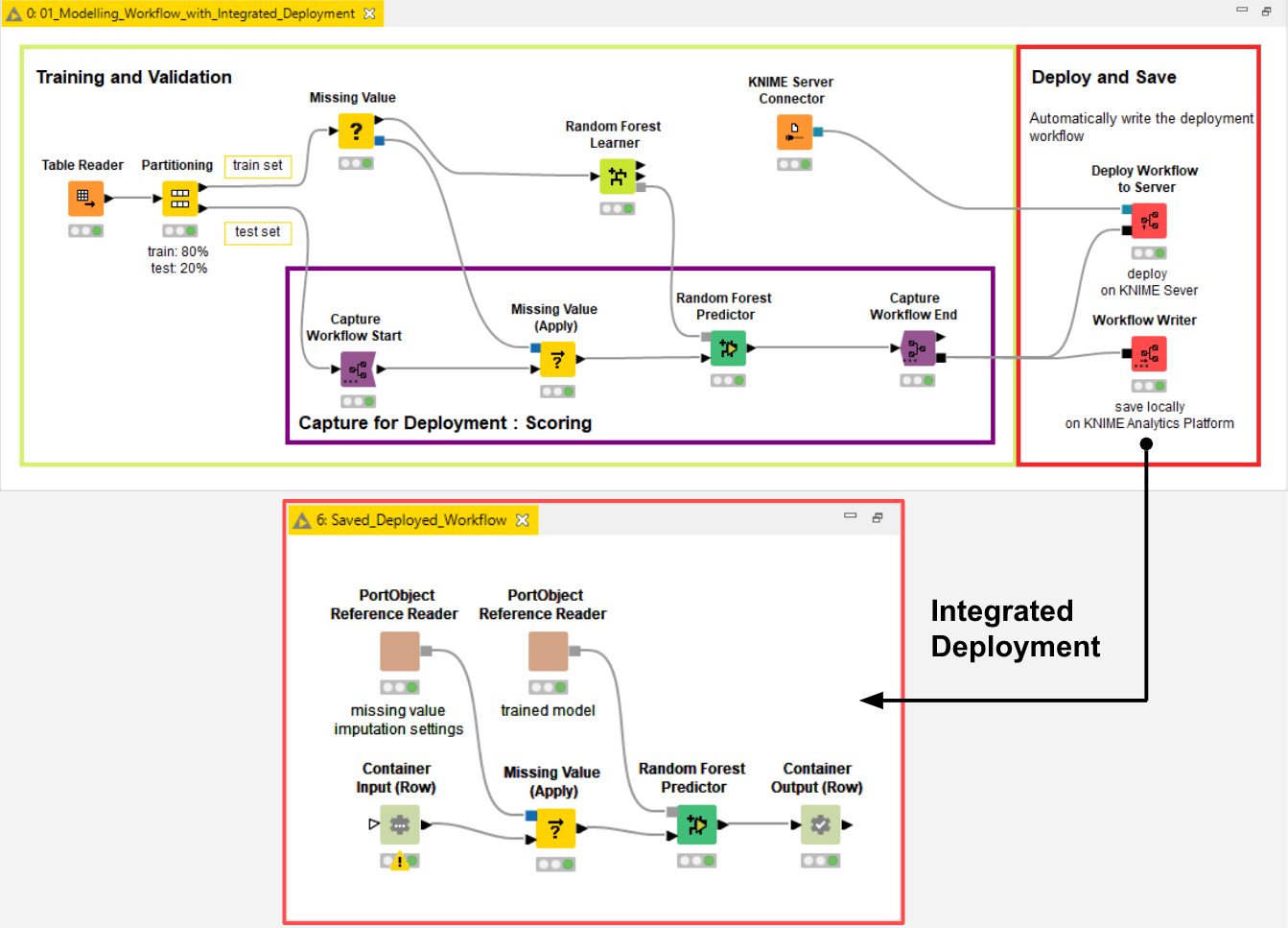
With Integrated Deployment, all of this has become easier, because you can control the data transformations in both training and production workflows from a single workflow. The KNIME Integrated Deployment extension allows you to capture a workflow segment - with the Capture Workflow Start and Capture Workflow End node - and automatically replicates it in a new workflow located on a KNIME Server via the Deploy Workflow to Server node or on the local workspace via the Workflow Writer node (Fig. 2).
This workflow subsequently becomes available for execution within your workflow list. All new changes in the captured segment are automatically reflected in the replica inside the new workflow.
You can now see how this extension can be used for the automatic generation of a production workflow. Identification of the relevant parts of the original workflow and automatic transfer into a second workflow prevents errors creeping into the deployment procedure.
As we have said, classic usage of Integrated Deployment refers to the deployment of production workflows containing machine learning models. But any production workflow in need of replicating a segment from an original workflow can benefit from Integrated Deployment.
To dive deeper into the details of how Integrated Deployment eases the deployment procedure job, we recommend the blog post “An introduction to Integrated Deployment”, which compares the old fashioned way of deploying production workflows with the new Integrated Deployment technique.
2. Execution of Workflow Segments for Model Monitoring
In the previous section, the generated workflow is stored in a selected folder and can be opened and executed from either KNIME Analytics Platform - if stored via a Workflow Writer node - or from a KNIME Server - if stored via a Deploy Workflow to Server node.
In this second example, we execute the captured segment from an entirely new workflow using the Workflow Executor node.
The application that we propose here has to do with model monitoring. If the model was correctly validated as part of the usual data science steps (for example as described in the CRISP-DM), its performance during production should be satisfactory. However, the good quality of the model does not last forever. There is rarely the guarantee that the data distribution won’t change. Model performance tends to slowly deteriorate over time. Therefore once a model is deployed, it needs to be monitored. If performance falls below a given threshold, model retraining must be triggered.
We use model monitoring in our Guided Analytics application implemented by the “Model Monitoring with Integrated Deployment” workflow. The application monitors the performance of a deployed production workflow containing the ML model. The current performance of each model is measured and visualized over time with the Model Monitor View component. This component includes two parts which handle:
- Calculation of the model predictions
- Evaluation and display of the model performance
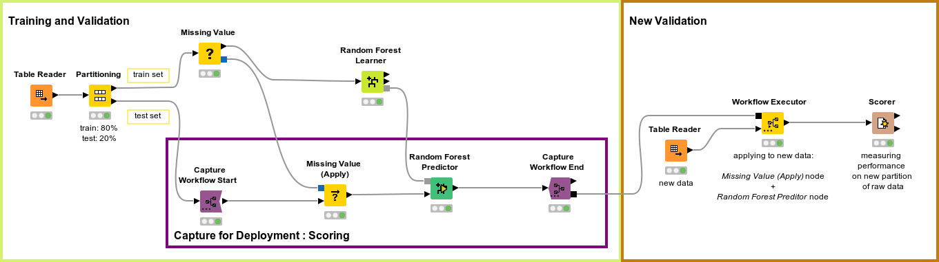
Calculation of the model predictions is implemented by a production workflow, created by capturing a specific workflow segment of the training workflow with Integrated Deployment. This captured segment is executed within the component by means of the Workflow Executor node (Fig. 3). The Workflow Executor node executes the workflow stored as Workflow Object at its input connection (black square port). This workflow object is what is usually output by Integrated Deployment nodes, such as a Capture Workflow End node.
The composite view of the Model Monitor View component includes a button to trigger the retraining of the model.
A similar component, the Model Monitor View (Compare) component, visualizes the performance of the newly re-trained model as compared to the old one. Its composite view also offers a button for updating the currently deployed production workflow with one containing the re-trained model (Fig. 4). (The workflow used in Fig. 4 is Model Monitoring with Integrated Deployment, available on the KNIME Hub.)
Notice that Integrated Deployment links the captured segment and its execution within the component. This means that if, for example, the predictor part in the captured segment changes, the generated predictions output by the Workflow Executor node change accordingly. The flexibility of this approach ensures that deployment is always correct and up to date.
3. Building a Black-Box Predictor
In the previous example, we executed the predictor part of our training workflow within a component in order to create the predictions on new data. Well, we can now push this a little further and use Integrated Deployment to create a black-box predictor.
In this case, our production workflows containing models would be represented as black boxes. A black box can be used totally ignoring what is inside by simply providing an input and receiving an output in return. A black box can be anything from a simple math formula to a complex deep learning model. Components and workflows using this black box approach tend to be preferred because they can work with any production workflow containing any ML algorithm or KNIME node.
The Model Monitor components in the previous section are good examples: via a black-box approach they can monitor any classification model. By executing the production workflow captured from the training workflow, we have de facto built a black-box predictor. We change the trained model and the predictor node in the captured segment and the output predictions change accordingly.
Using a black box approach on a production workflow gives you lots of flexibility when building and reusing model-agnostic workflows and components. Note you can always open the black box and visually explore the underlying production workflow via a Workflow Writer node.
We could further use these predictions to:
- Explain the black box via Machine Learning Interpretability (MLI) techniques;
- Produce conformal predictions from a black box to determine precise levels of confidence in new predictions;
- Combine them with predictions from other models to form an ensemble model;
- Validate the performance of the black box production workflow.
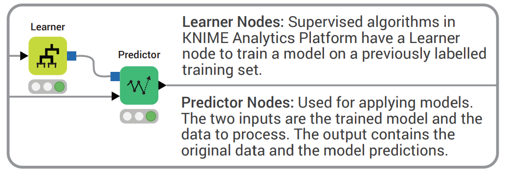
Remember the Learner-Predictor tandem in KNIME Analytics Platform? The Learner node trains the model, the Predictor node applies the model (Fig. 5).
KNIME has a range of cheat sheets you can view online and also download, in addition to the KNIME Beginner Cheat Sheet, you will find cheat sheets for Control and Orchestration in KNIME Analytics Platform and a Machine Learning Cheat Sheet too. You will find them all on Cheat Sheet webpage.
As per Integrated Deployment, you can recreate a Learner and a Predictor node to consume any machine learning algorithm. In this case, one Workflow Executor node plays the Learner role by embedding the learner segment and one other Workflow Executor node plays the Predictor role by embedding the predictor segment from the original workflow.
As we said, this approach fits any machine learning algorithm. Furthermore, your learner or predictor Workflow Executor node can now enclose a full workflow segment, as it can also include a more complex structure with several nodes (normalization, missing value imputation, ..) than just a simple Predictor node.
The Workflow Executor node has dynamic input ports. By default only one input port is available (the black square for the captured segment). However, new input ports are automatically added when trying to connect a data port to it (Fig. 6).
A great example of this learner-predictor framework can be seen in the XAI View. This component is used in the workflow “eXplainable Artificial Intelligence (XAI)” and explains the production workflow provided at its input as a black box, using both local and global machine learning interpretability (MLI) techniques: shapley values, partial dependence and a surrogate decision tree. The black-box model is provided at the input port of this component via the black square port, accepting production workflows captured via Integrated Deployment.
By adopting the Workflow Executor node as a black-box predictor you can build workflows and components as model-agnostic techniques: compatible with any ML algorithm captured in a black box via Integrated Deployment.
4. Freezing Settings from Interactive Views for Reproducibility
Some components in complex automation workflows include an interactive view to ease and guide the user through the analytics procedure. The user is able to interact via the component view and when satisfied with the results she can apply those final settings to export the consequent results into a data table.
When this kind of operation is performed on a routine basis it must be possible to re-execute the component using the same settings the user made in her last interaction - for the purposes of reproducibility and auditing.
So wouldn't it be nice to export that part of the component as it was last used? Such workflow segments could be inspected, understood, and re-executed on-demand.
With the Integrated Deployment nodes we can implement a component with this reproducible framework. Its new settings are inherited from the last used interactive view. Once the component’s interactive view is closed, and the interactions saved, the component exports:
- A data table with the results from the input data
- A small workflow segment, stored in a workflow object, with settings inherited from the last interaction in the interactive view, reproducing the same results for the same input data, and executing on demand on other samples of data
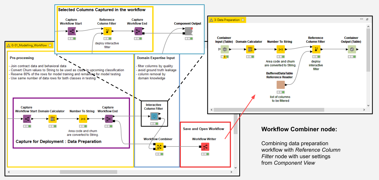
An example of this approach has been implemented with the Interactive Column Filter verified component in the workflow Automated Visualization with Interactive Column Filter. In the interactive View of this component the user can quickly explore the results of some column filtering operations and then re-execute the component with the settings saved after the last exploration by means of the Workflow Executor node.
This approach can be used for a variety of use cases, for example to document execution for auditing purposes and to guarantee the reproducibility of the execution session. Freezing workflows based on interactive views can be extremely helpful to reproduce experiments, for debugging, and to automate user interactions.
Just before we move on to our fifth example of how Integrated Deployment can be used, we would like to draw your attention to two separate segments in this workflow that were captured and combined using Integrated Deployment. The idea here is to demonstrate how the Workflow Combiner node can be used to capture and combine workflow segments into a single, automatically generated workflow (Fig. 7).
5. Code Generating Code
Ultimately, Integrated Deployment is about automatically and dynamically defining a function as a workflow segment with inputs, outputs, and parameters, etc. Users can design a new generation of workflows that are able to self update, automatically change configuration settings, and trigger a chain reaction of workflows writing workflows writing workflows.
An example of this can be seen in the Continuous Deployment workflow (Fig. 8) for a simple Continuous Integration / Continuous Deployment (CI/CD) example in data science. The workflow creates a workflow, which creates yet another workflow in order to change which model is trained and still be able to redeploy without editing any workflow node. You can find more details on the Continuous Deployment blog post.
Practically Integrated Deployment is a way of recycling workflow segments, by isolating interesting parts in the original workflow and dynamically replicating them in a new workflow. In this way, we can define functions correctly, by reliably reusing existing workflows, and dynamically, by just replicating the segments with all the related changes over time. This is code generating new code within the KNIME visual programming framework.
Integrated Deployment Provides Multipurpose Functionality
In this article we have looked at five ways to use the KNIME Integrated Deployment extension. We started with the automated creation of a production workflow; we then moved to the execution of workflow segments; based on that, we built a black-box predictor; we executed components after freezing their settings from visual inspection; and finally we used Integrated Deployment as a means to reliably generate new workflows by recycling old workflows.
We have seen how important Integrated Deployment is to ease and maintain the deployment of models, but we have also seen it in action in other situations not directly related to deployment. These five possible ways of using Integrated Deployment are only a subset of what’s possible and it’s up to your creativity to build more complex workflows to reliably process and output workflow objects.
The Integrated Deployment KNIME Blog Articles
Explore the collection of articles on the topic of Integrated Deployment.