A tutorial on KNIME Deeplearning4J Integration

The aim of this blog post is to highlight some of the key features of the KNIME Deeplearning4J (DL4J) integration, and help newcomers to either Deep Learning or KNIME to be able to take their first steps with Deep Learning in KNIME Analytics Platform.

If you’re new to KNIME, here is a link to get familiar with the KNIME Analytics Platform:
KNIME Courses: self paced, online, or onsite

If you’re new to Deep Learning, there are plenty of resources on the web, but these two worked well for me:
https://deeplearning4j.org/neuralnet-overview
http://playground.tensorflow.org/

If you are new to the KNIME nodes for deep learning, you can read more in the relevant section of the Node Guide:
https://www.knime.com/nodeguide/analytics/deep-learning

With a little bit of patience, you can run the example provided in this blog post on your laptop, since it uses a small dataset and only a few neural net layers. However, Deep Learning is a poster child for using GPUs to accelerate expensive computations. Fortunately DL4J includes GPU acceleration, which can be enabled within the KNIME Analytics Platform.

If you don’t happen to have a good GPU available, a particularly easy way to get access to one is to use a GPU-enabled KNIME Cloud Analytics Platform, which is the cloud version of KNIME Analytics Platform, available on both AWS and Azure.

In the addendum at the end of this post we explain how to enable KNIME Analytics Platform to run deep learning on GPUs either on your machine or on the cloud for better performance.

We will use the MNIST dataset. The MNIST dataset consists of handwritten digits , from 0 to 9, as 28x28 pixel grayscale images. There is a training set of 60,000 and a test set of 10,000 images. The data are available from:
http://yann.lecun.com/exdb/mnist/

Our workflow downloads the datasets, un-compresses them, and converts them to two CSV files: one for the training set, one for the test set. We then read in the CSV files, convert the image content to KNIME image cells, and then use the KNIME DL4J nodes to build a variety of classifiers to predict which number is present in each image.

We aim at an accuracy of >95%, according to the error rates listed in the original article by Le Cun et al..

The workflows built throughout this blog post are available on the KNIME EXAMPLES Server under 04_Analytics/14_Deep_Learning/14_MNIST-DL4J-Intro04_Analytics/14_Deep_Learning/14_MNIST-DL4J-Intro^*. This workflow group consists of:

• The workflow named DL4J-MNIST-LeNet-Digit-Classifier
• The “data” workflow group to contain the downloaded files
• The “metanodes” workflow group which contains the three metanode templates used in the example.

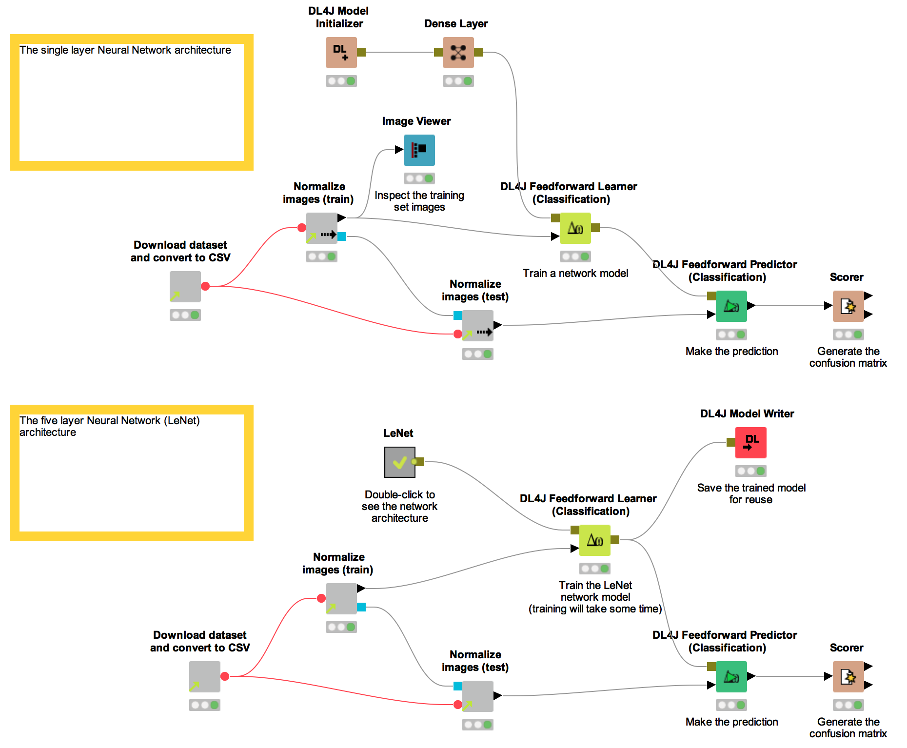
The workflow named DL4J-MNIST-LeNet-Digit-Classifier (Fig. 1) actually consists of 2 workflows: the top one uses a simpler net architecture, while the lower one uses a 5 layer net architecture.

Figure 1. Workflows created during this blog post and available on the KNIME EXAMPLES server under 04_Analytics/14_Deep_Learning/14_MNIST-DL4J-Intro. This workflow actually consists of 2 workflows: the top one using a simpler deep learning architecture; the lower one using a 5 layer deep learning network.

We ran the whole experiment using a KNIME Cloud Analytics Platform running on an Azure NC6 instance. Of course, you can equally run it on an Amazon Cloud p2.xlarge instance or your local machine.

Beware. This workflow could take around an hour to run, depending on whether you have a fast GPU, and how powerful your machine is!

Tools:

1. KNIME Analytics Platform 3.3.1 (or greater) on your machine
   OR
   KNIME Cloud Analytics Platform on Azure Cloud
   OR
   KNIME Cloud Analytics Platform on AWS Cloud
2. Python 2.7.x configured for use with KNIME Analytics Platform:
   https://www.knime.org/blog/how-to-setup-the-python-extension

Extensions:

• KNIME Deeplearning4J extension from KNIME Labs Extensions/KNIME Deeplearning4J Integration (64 bit only).
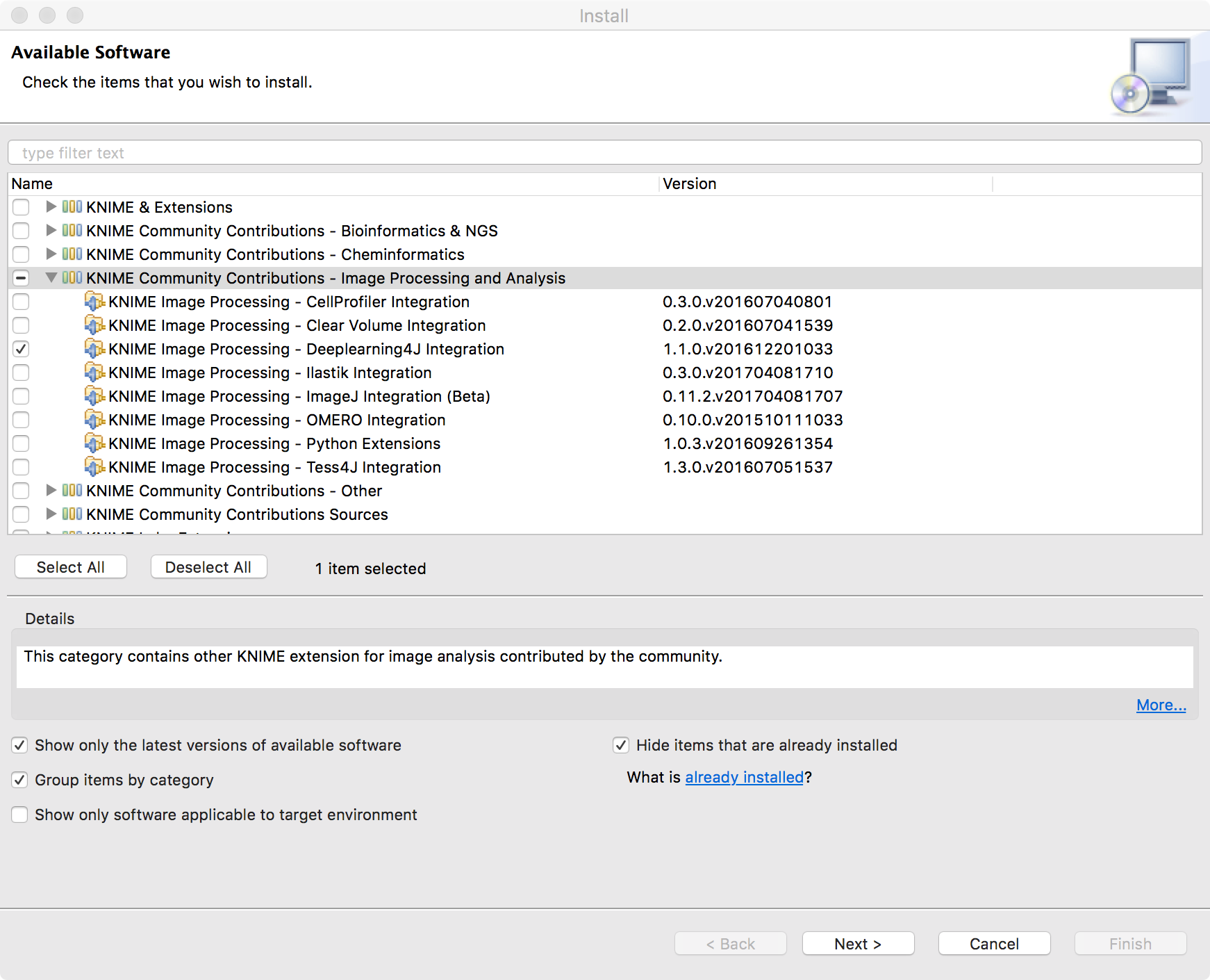
• KNIME Image Processing extension from the KNIME Community Contributions - Image Processing and Analysis
• KNIME Image Processing - Deep Learning 4J Integration
• Vernalis KNIME Nodes from KNIME Community Contributions - Cheminformatics
• KNIME File Handling Nodes and KNIME Python Integration from KNIME & Extensions

If you are running KNIME Analytics Platform on your machine:

• KNIME Image Processing - Deeplearning4J Integration from the Stable Community Contributions update site (note this update site must be manually enabled, see Addendum for details)

Optionally, if you have GPUs:

• GPU support

Often when working with images, it is possible to read them directly in KNIME Analytics Platform from standard formats like PNG, JPG, TIFF. Unfortunately for us, the MNIST dataset is only available in a non-standard binary format. Luckily, it is straightforward to download the dataset and convert the files to a CSV format that can be easily read into KNIME.

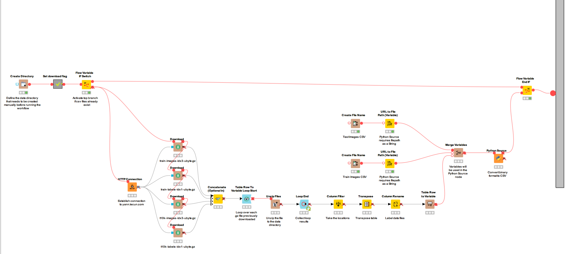
The data import is handled by the ‘Download dataset and convert to CSV’ metanode. Here the data files are downloaded from the LeCunn website, and written to the folder named “data” and contained in the workflow group 14_MNIST-DL4J-Intro that you have downloaded from the EXAMPLES server.

In order to extract the pixel values for each image, we use a Python Source node to read the binary files and output to two CSV files (mnist_test.csv, mnist_train.csv). We have implemented an IF statement that only downloads and converts the files if the mnist_test.csv and mnist_train.csv files do not already exist; there’s no sense doing that download twice!

Figure 2. Content of the metanode named "Download dataset and convert to CSV". This metanode downloads the data files and writes them to a local "data" folder. Then through a Python Source node converts the binary pixel content into a CSV file.

Now we have numerical columns representing images. In the wrapped metanode named “Normalize images (train)” (Fig. 3), a File Reader reads the numerical columns and normalizes them with a Normalizer node.

The conversion back into binary images is obtained via the Data Row to Image node from the KNIME Image Processing extension. The Deeplearning4J (DL4J) integration in KNIME can handle numbers, strings, collections, or images (when the KNIME Image Processing - Deep Learning 4J extension is installed from the stable community update site) as input features.

It is important to randomize the order of the input rows, in order not to bias the model training with the input sequence structure. For that, we used the ‘Shuffle’ node.

Figure 3. Content of the "Normalize images (train)" wrapped metanode. Notice the execution in streaming mode and the transformation output port for the Normalization model.

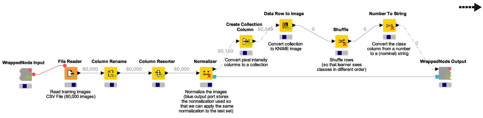
The normalization model produced by the Normalizer node is exported from the Wrapped Metanode. We do this so that we can re-apply the same normalization to the test dataset in the wrapped metanode named “Normalize images (test)”.

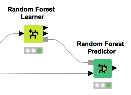
In addition to the typical KNIME Learner/Predictor schema, the DL4J Learner node requires a network architecture as input for the learning process (Fig. 4 vs. Fig. 5).

There are two ways to define a network architecture:

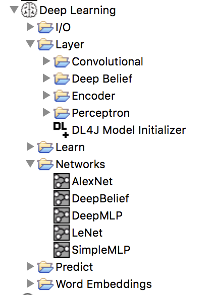
1. Select one from some well-known pre-built network architectures available under KNIME Labs/Deep Learning/Networks in the Node Repository
2. Build your own neural architecture from scratch.

Figure 6. Deep Learning/Networks sub-category contains a number of pre-built commonly used deep learning architectures.

Since we are experimenting, we will build our own network and we’ll start with a toy network.

We start with the DL4J Model Initializer node. We don’t need to set any options for this node. Next we introduce the Dense Layer. This time we need to set some options, but let’s stick with the default options for now, which creates the output layer with only one output unit to represent the numbers from 0 to 9, activation function ReLu, random weight initialization according to the XAVIER strategy, and a low learning rate value as 0.1. We have created the simplest possible (and not very deep!) neural network.

Now we can link our training set and the simple neural network architecture to the ‘DL4J Feedforward Learner (Classification)’ node. This learner node needs configuration.

The configuration window of the DL4J Feedforward Learner (Classification) node is somewhat complex, since it requires settings in 5 configuration tabs: Learning Parameter, Global Parameter, Data Parameter, Output Layer Parameter, and Column Selection. In general, there are many options available to set, the Deep Learning 4J website has some nice hints to help people get started.

The first 2 tabs, “Learning Parameter” and “Global Parameter” define the learning parameters used to train our network. Here since we are just getting started at this stage I accept the default options. The defaults are to use Stochastic Gradient Descent for optimizing the network. Nesterovs as the updater, with momentum of 0.9. We don’t set any global parameters, which would override those parameters set in the individual network layer node configuration dialogs. We’ll work on tuning the learning parameters in the LeNet workflow that we’ll get to shortly.

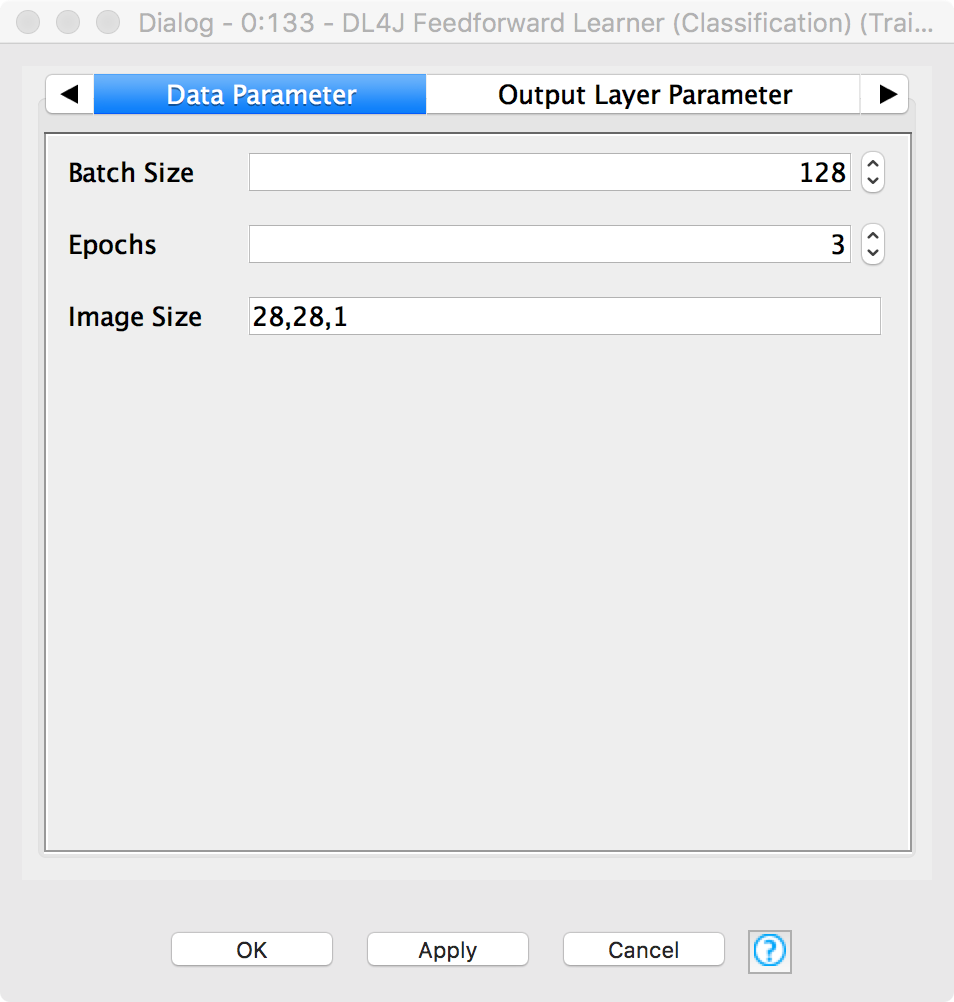
The third tab, named “Data Parameter”, defines how data is used to train the model. Here I set Batch Size to 128, Epochs to 15, and Image Size to 28,28,1. Batch size defines the number of images that are passed through the network and used to calculate the error, before updating the network. Larger batch sizes mean longer to wait between each update, but also give the possibility of learning more information with each iteration. Epochs describe the number of full passes of the dataset that are made, choices here can help to guard against under/over-fitting of the data. The image size is the size of the image in pixels (x,y,z).

Figure 7. The "Data Parameter" tab in the configuration window of the DL4J Feedforward Learner (Classification) node. Batch Size defines the number of images used for each network parameter update and is set to 128 as a trade off between accuracy and speed. Epochs are set to 3 since in this case we want the example to run for only a short time. Image Size defines the size of image on the x, y, z axis in number of pixels.

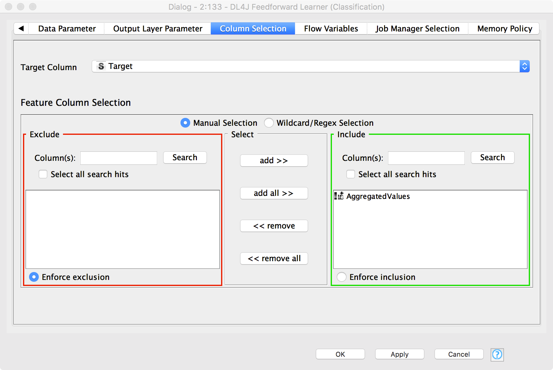
The ‘Column Selection’ tab contains all information about input columns and target column. The target column is set to column ‘Target’, which contains the number represented in the image. The image column named “AggregatedValues” is used as the input feature.

Figure 8. "Column Selection" tab in the configuration window of the DL4J Feedforward Learner (Classification) node. This tab sets the target column and the input columns.

Finally connecting up the corresponding Predictor and the Scorer nodes we can test the model quality (see upper workflow in figure 1).

To train our first not-so deep learning model, we need to execute the DL4J Feedforward Learner (Classification). The execution of this node can take some time (probably more than 10 minutes). However, it is possible to monitor the learning progress, and even to terminate it early, if a suitable model has already been reached. Right-clicking the DL4J Feedforward Learner (Classification) node and selecting ‘View: Learning Status’ from the context menu displays a window including the current training epoch and the corresponding Loss (=Error) calculated on the whole training set (Fig. 9). If the loss is sufficient for our purpose or if we have become impatient, we can hit the “Stop Learning” button to stop the training process.

Once the calculation is complete you can execute the Scorer node to evaluate the model accuracy (Fig. 10).

Figure 9. Learning Status window for the DL4J Feedforward Learner (Classification) node. This window is open by right-clicking the node and selecting the option " View: Learning Status". Here you can monitor the learning progress of your deep learning architecture. You can also stop it at any moment by hitting the “Stop Learning” button.

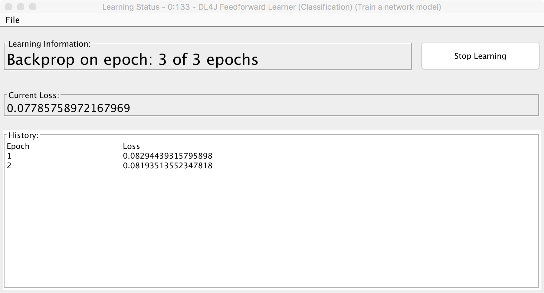
Figure 10. Confusion Matrix and Accuracy of the single-layer neural network trained on the number data set to recognize numbers in images. Notice the disappointing ~35% Accuracy. A single-layer network is not enough?

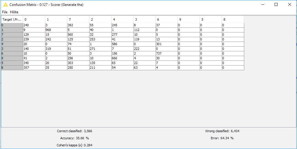
Did you notice the accuracy just a little above 35%? That was a little disappointing! But not entirely unexpected. We didn’t spend any time optimizing the input parameters since we’re not aiming to evaluate what the optimal network architecture is, rather to see how easy it is to reproduce one of the more well known complex architectures. It is well known that deep learning networks often require several layers and careful optimization of input parameters. So in order to go a bit deeper, in the next section we’re going to take the LeNet network that has been pre-packaged in the Node Repository, and use that.

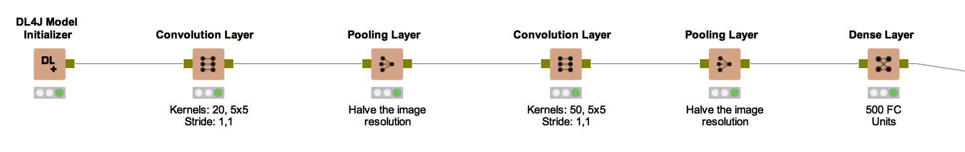
We can quickly import a well-known architecture that has been shown to work well for this problem by dragging and dropping the ‘LeNet’ metanode from the Node Repository into the workspace. Double-clicking the “LeNet” metanode lets us take a look at the network topology. We see that there are now five layers defining the network (Fig. 11).

The process of building the network architecture is triggered again by a “DL4J Model Initializer” node, requiring no settings. We then add a Convolution Layer (which applies a convolution between some filter with defined size to each pixel in the image), a Pooling Layer (pooling layers reduce the spatial size of the network - in this case halving the resolution at each application), then again a Convolution Layer, a Pooling Layer, and a Dense Layer (neurons in a dense layer have full connections to all outputs of the previous layer). The result is a 5-layer neural network with mixed types of layers.

Figure 11. LeNet neural network architecture as built in the "LeNet" metanode.

Finally we make a few more changes in order to closely match the parameters originally described in the article by LeCun et al.. That means setting the learning rate to 0.001 in the DL4J Feedforward Learner (Classification) node. The Output Layer parameters are 0.1 learning rate, XAVIER weight initialisation and Negative Log Likelihood loss function.

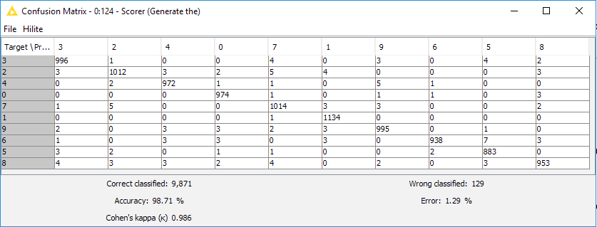
Evaluating the results we can clearly see that adding the layers and tweaking the parameters has made a huge difference in the results. We can now predict the digits with 98.71% accuracy!

Figure 12. Confusion Matrix and Accuracy of a neural network shaped according to the LeNet architecture, that is introducing 5 hidden mixed type layers in the network architecture. The network is trained again on the number data set to recognize numbers in images. Now we get almost 99% Accuracy. This is much closer to the performances obtained by LeCun et al..

Deep Learning is a very hot topic in machine learning at the moment, and there are many, many possible use cases. However, you’ll need to spend some time to find the right network topology for your use case and the right parameters for your model. Luckily the KNIME Analytics Platform interface for DL4J makes setting those models up straightforward.

What’s more, the integration with KNIME Image Processing allows you to apply Deep Learning to image analysis, and using the power of GPUs in the cloud, it might not take as long as you think to get started.

To enable KNIME Analytics Platform to run deep learning using GPUs, follow the instructions reported in the final part of the addendum.

Perhaps, more importantly than that, it is also easy to deploy those models using the WebPortal functionality of the KNIME Server, but that discussion is for another blog post…

Tweet me: @JonathanCFuller

1. http://yann.lecun.com/exdb/mnist/
2. http://yann.lecun.com/exdb/publis/pdf/lecun-98.pdf

Workflows:

• the workflow used for this blog post is available on the KNIME EXAMPLES Server at 04_Analytics/14_Deep_Learning/14_MNIST-DL4J-Intro04_Analytics/14_Deep_Learning/14_MNIST-DL4J-Intro^*

---

With KNIME Cloud Analytics Platform pre-configured and available via the AWS and Azure Marketplaces it is straightforward to run DL4J workflows on a GPU.

Note that to see a speedup in your analysis you’ll need to have a modern GPU designed for Deep Learning, which is exactly what the Nvidia K80 GPUs available on Azure NC6 instances and AWS P1 instances are.

If you have a modern GPU on your local machine, you can also run the GPU enabled workflows using a KNIME Analytics Platform installation on your local machine.

In this addendum we offer a step by step guide on what to install and what to enable to run deep learning on a KNIME Analytics Platform, optionally using GPU acceleration and a cloud installation.

1. On a Cloud Instance
   Launching KNIME Cloud Analytics Platform differs slightly in each of the marketplaces, but the following documents show how to launch an instance.
   1. Azure NC6 instances
      Note that at the time of writing NC6 instances are only available in the following regions: East US, South Central US, West US 2. See here for latest availability: https://azure.microsoft.com/en-us/regions/services.
      Note also that the KNIME DL4J integration currently only supports single GPU machines, so choose NC6 instances rather than the instances with multiple GPUs.
   2. AWS P2.xlarge instances.
2. On your Machine.
   Follow these instructions for:
   • Windows https://youtu.be/yeHblDxakLk
   • Linux https://youtu.be/wibggQYr4ZA
   • Mac https://youtu.be/1jvRWryJ220

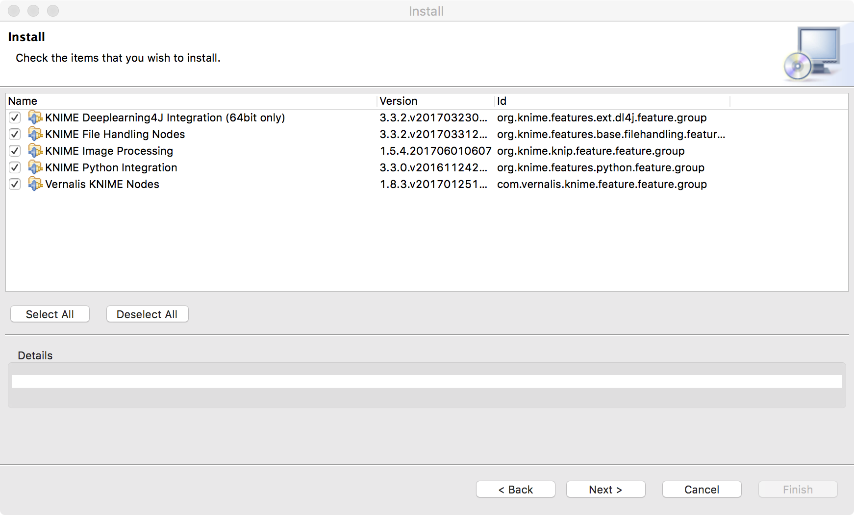
When you load a workflow, KNIME Analytics Platform checks that all required extensions are installed. If any are missing, you will be prompted to install them (Fig. 13). Choosing Yes, will start the installation process for the missing extensions. We recommend to install all missing extensions for this workflow (Fig. 14).

Note. Missing nodes in a workflow are visualized via a red and white grid icon. If your workflow still has missing nodes and you are prompted to save it, you should choose ‘Don’t save’.

Figure 13. Prompt to install missing KNIME extensions.

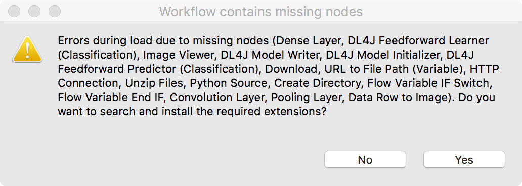
Figure 14. Recommended KNIME Extensions to install to run the workflow described in this blog post

If you are not prompted or if you have saved the workflow with missing nodes, you can still install the missing extensions manually. Following the instructions in this YouTube video https://youtu.be/8HMx3mjJXiw, install:

• KNIME Deeplearning4J extension from KNIME Labs Extensions/KNIME Deeplearning4J Integration (64 bit only).
• KNIME Image Processing extension from the whole KNIME Community Contributions - Image Processing and Analysis
• Vernalis KNIME Nodes from KNIME Community Contributions - Cheminformatics
• KNIME File Handling Nodes and KNIME Python Integration from KNIME & Extensions

Note that if your extension is already installed you will probably not see it in the list of installable packages.

After installation, you should have the following categories in the Node Repository: Deep Learning under KNIME Labs, KNIME Image Processing and Vernalis under Community Nodes, Python under Scripting, File Handling under IO.

In order to use the KNIME Python integration, you need Python 2.7.x configured for use with KNIME Analytics Platform. Follow the instructions described in this blog post: https://www.knime.org/blog/how-to-setup-the-python-extension

If you rely on existing installations of KNIME extensions, it might happen that you are still missing the specific KNIME Image Processing support for DL4J Integration, since this is a quite new component.

To manually install the KNIME Image Processing support for DL4J Integration extension, follow these steps.

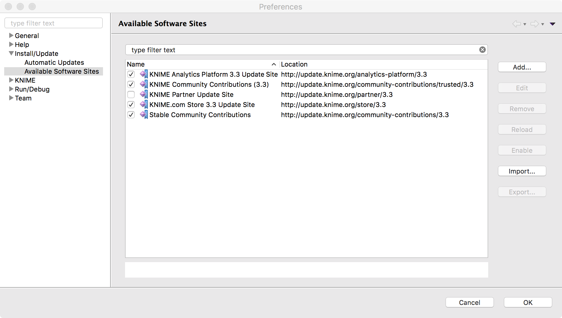
1. File > Preferences, and enable the ‘Stable Community Contributions Update Site’

Figure 15. Enable "Stable Community Contributions Update" site. it is not enabled by default.

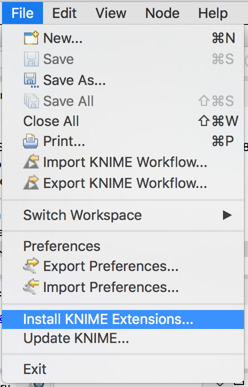
1. File > Install KNIME Extensions…

Figure 16. "Install KNIME Extensions ..." option from File Menu

1. Install KNIME Image Processing – Deeplearning4J Integration

Figure 17. Install KNIME Image Processing - Deeplearning4J Integration

1. Configure CUDA support
   Once you’ve logged into your newly launched KNIME Cloud Analytics Platform instance, you’ll need to install the CUDA libraries required for the DL4J GPU support. That is described here:
   http://docs.nvidia.com/cuda/cuda-installation-guide-microsoft-windows/index.html#axzz4ZcwJvqYi
   Use this download link:
   https://developer.nvidia.com/compute/cuda/8.0/Prod2/local_installers/cuda_8.0.61_win10-exe
2. Enable KNIME Analytics Platform to use GPUs
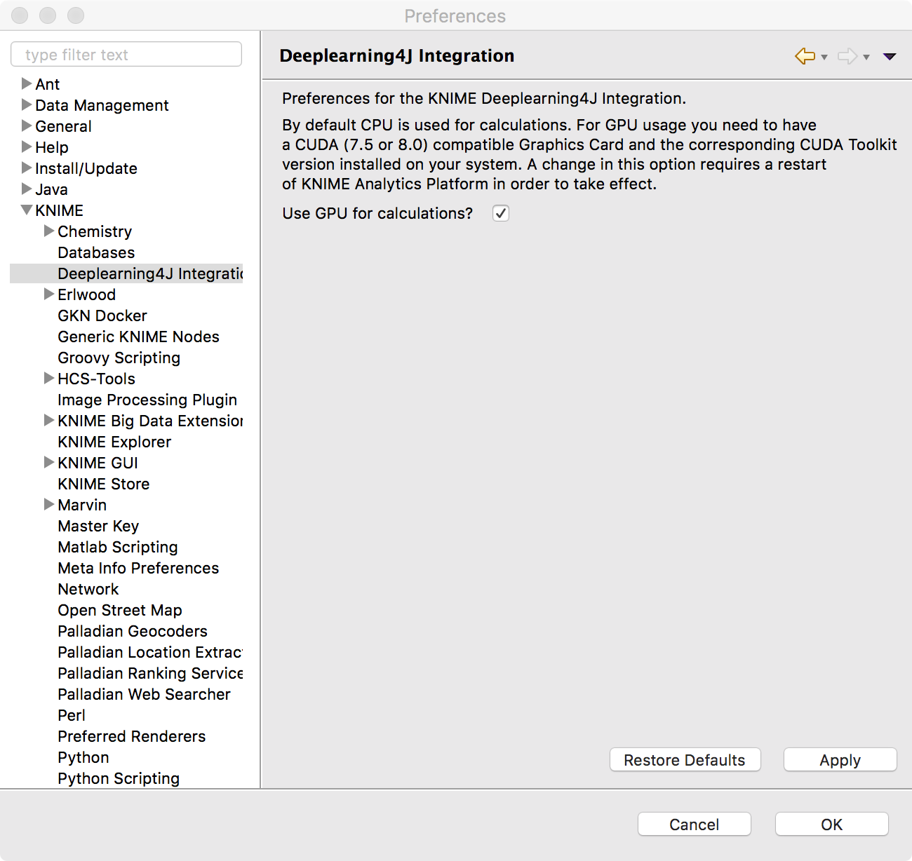
   Finally you’ll need to enable the Deeplearning4J Integration GPU support. That can be found under File > Preferences, and then searching for Deeplearning4J Integration. You’ll need to check the box ‘Use GPU for calculations?’. Don’t restart your Analytics Platform just yet, there is one more step required.

Figure 18. Enable usage of GPU for deep learning in the Preferences page

---

* The link will open the workflow directly in KNIME Analytics Platform (requirements: Windows; KNIME Analytics Platform must be installed with the Installer version 3.2.0 or higher)