
The ability to automatically analyze customer feedback helps businesses process huge amounts of unstructured data quickly, efficiently, and cost effectively. That’s why sentiment analysis is used widely as a marketing analytics tool, for example to measure consumer sentiment about products, services, or brands. This article is part of a series on how to automate sentiment analysis with KNIME.
Today we show how to use a popular deep learning architecture, tailored for sequential data, to learn and predict the sentiments in US airlines’ reviews. Approaches for sentiment analysis have advanced from simple rules to advanced machine learning, and deep learning techniques. Deep learning techniques have proven to be superior in analyzing and representing complex language structures.
Understand LSTM-based neural networks
Imagine that you want to classify what kind of event is happening at every point in a movie. Traditional neural network architectures are not well suited for this task, since it is unclear how their reasoning about previous events in the film could be used to inform later ones [1]. On the other hand, Recurrent Neural Networks (RNNs) are great at addressing this task because they have node connections that form a graph along a sequence of data, mimicking memory and allowing information to persist.
RNNs are also a great candidate for sentiment analysis of text because they are capable of processing variable-length input sequences, such as words and sentences. In fact, RNNs have shown great success in many sequence-based problems, such as text classification and time series analysis.
Most of this success, however, is linked to a very special kind of RNN: LSTM-based Neural Networks. The performance of the original RNNs decreases as the gap between previous relevant information and the place where it is needed grows. Imagine you are trying to predict the last word in the sentence “The clouds are in the sky”. Given this short context window, it is extremely likely that the last word is going to be sky. In such cases, where the gap between the context and the prediction is small, RNNs perform consistently well. As this gap grows, which is very common in more complex texts, it is better to use LSTMs. The reason why LSTMs are so good at keeping up with larger gaps has to do with their design: just like traditional RNNs, they also have a graph-like structure with repeating modules, but LSTMs are more complex and tackle longer-term dependencies much better.
Read more about the structure of LSTMs and RNNs in the article “Once Upon a Time …” by LSTM Network.
Now Perform LSTM-based Sentiment Analysis in KNIME
The goal of our article is to build a predictor for sentiments (positive, negative, or neutral) in US airline reviews. To train and evaluate the predictor, we use a Kaggle dataset with over 14K customer reviews in the format of tweets, which are annotated as positive, negative, or neutral by contributors. The closer the predicted sentiments are to the contributors’ annotations, the more efficient our predictor is.
You can find the workflows for this project, in which we build and deploy a LSTM-based predictor for sentiment analysis, in the Machine Learning and Marketing space on the KNIME Hub. The most relevant parts of the workflows are detailed below.
Preliminary Steps – KNIME Keras or Python Integration
In order to execute the workflows that we are going to discuss today, you will need to:
- Install the KNIME Deep Learning - Keras Integration extension
- Use the Conda Environment Propagation node for the workflows in this tutorial, which ensures the existence of a Conda environment with all the needed packages. An alternative to using this node is setting up your own Python integration to use a Conda environment with all packages.
Note: These workflows were tailored for Windows. If you execute them on another system, you may have to adapt the environment of the Conda Environment Propagation node.
Tip: You can find more information on using the Keras Integration in this article about text generation with LSTMs.
How to define the neural network architecture
We start our solution by defining a neural network architecture to work with. In particular, we need to decide which Keras layers to use and in what order.
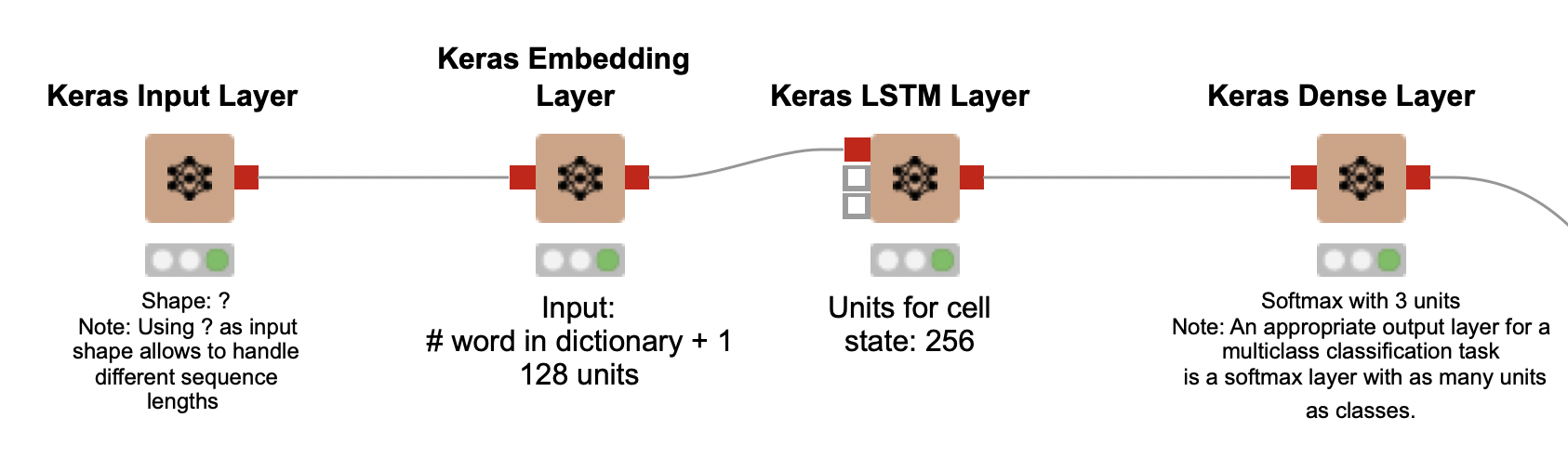
Keras Input layer
In KNIME, the first layer of any Keras neural network, which receives the input instances, is represented with the Keras Input Layer node. In our application, the input instances are tweets. This layer requires a specification of the input shape, but since our instances are tweets with varying numbers of words (that is, with varying shapes), we set the parameter shape as “?”. This allows the network to handle different sequence lengths.
Keras Embedding layer (and why we need one)
After an instance is processed in the input layer, we send it to the Keras Embedding Layer node, which encodes the tweets into same-sized representations (embeddings). Working with same-sized sequences is going to be important when we get to the training part of our workflow. In general, RNNs can handle sequences with different lengths, but during training they must have the same length.
To understand what this layer does, let’s first discuss a very naive way of representing tweets as embeddings. The tweets in this project use a vocabulary with a large number X of words, and we could easily create an X-sized vector to represent each tweet, such that each index of the vector would correspond to a word in the vocabulary. In this setting, we could fill these vectors as follows:
- For each word that is present in a tweet, set its corresponding entry in the tweet’s X-sized vector as 1;
- Set all the other vector entries as 0.
This is a very traditional way of encoding text, and leads to same-sized representations for the tweets regardless of how many words they actually contain.
Enter the embedding layer! It receives these X-sized vectors as input and embeds them into much smaller and denser representations, which are still unique – that is, two different tweets will never be embedded in the same way. Here, we configure the Keras Embedding Layer node by setting two parameters: the input dimension and the output dimension. The input dimension corresponds to the total number of words present in the set of tweets – that is, the vocabulary – plus one. We will explain how to determine this value later on in this article, but it basically depends on the native encoding of your operating system. In Windows, the vocabulary size for our tweet dataset is calculated as 30125, so we set the input dimension as 30126. The output dimension corresponds to the size of the embeddings, and we set it as 128. This means that regardless of how many words each tweet originally has, it will be represented as an embedding (you can see it as a vector) of size 128. A massive economy in how much space is used!
The larger the embeddings are, the slower your workflow will be, but you also do not want to use a size that is very small if you have a large vocabulary and many tweets: for our application, size 128 hits the spot.
LSTM layer
We connect the Keras Embedding Layer node to the star of our neural network: the Keras LSTM Layer node. When configuring this layer, we need to set its number of units. The more units this layer has, the more context is kept – but the workflow execution also becomes slower. Since we are working with short text in this application (tweets), 256 units suffice.
Dense layer
Finally, we connect the Keras LSTM Layer node to a Keras Dense Layer node that represents the output of our neural network. We set the activation function of this layer as softmax to output the sentiment class probabilities (positive, negative, or neutral) for each tweet. The use of softmax in the output layer is very appropriate for multiclass classification tasks, with the number of units being equal to the number of classes. Since we have 3 classes, we set the number of units in the layer as 3.
Preprocess the data before building the predictor
Before building our sentiment predictor, we need to preprocess our data. After reading our dataset with the CSV Reader node, we associate each word in the tweets’ vocabulary with an index. In this step, which is implemented in the Index Encoding and Zero Padding metanode, we break the tweets into words (tokens, more specifically) with the Cell Splitter node. Read more about different encoding options in this review on text encoding.
Here is where the native encoding of your operating system may make a difference in the number of words you end up with, leading to a larger or smaller vocabulary. After you execute this step, you may have to update the parameter input dimension in the Keras Embedding Layer to make sure that it is equal to the number of words extracted in this metanode.
Since it is important to work with same-length tweets in the training phase of our predictor, we also add zeros to the end of their encodings in the Index Encoding and Zero Padding metanode, so that they all end up with the same length. This approach is known as zero padding.
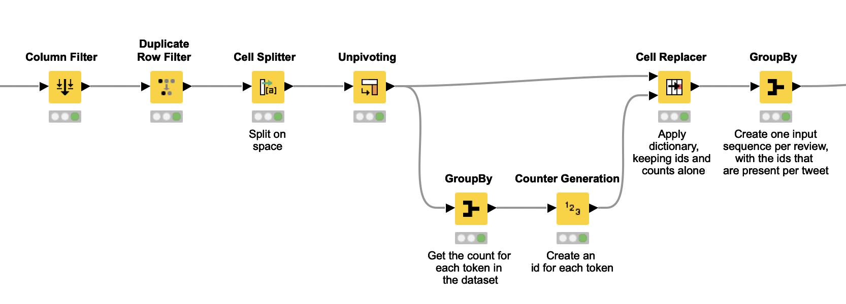
Already outside of the metanode, the next step is to use the Table Writer node to save the index encoding for the deployment phase. Note that this encoding can be seen as a dictionary that maps words into indices.
The zero-padded tweets output by the metanode also come with their annotated sentiment classes, which also need to be encoded as numerical indices for the training phase. To do so, we use the Category to Number and the Create Collection Column nodes. The Category to Number node also generates an encoding model with a mapping between sentiment class and index. We save this model for later use with the PMML Writer node.
Finally, we use the Partitioning node to separate 80% of the processed tweets for training, and 20% of them for evaluation.
Train and apply the neural network
With our neural network architecture set up, and with our dataset preprocessed, we can now move on to training the neural network.
To do so, we use the Keras Network Learner node, which takes the defined network and the data as input. This node has four tabs, and for now we will focus on the first three: the Input Data, the Target Data, and the Options tabs.
In the Input Data tab, we include the zero-padded tweets (column ColumnValues) as input. In the Target Data tab, we use column Class as our target and set the conversion parameter as “From Collection of Number (integer) to One-Hot-Tensor” because our network needs a sequence of one-hot-vectors for learning.
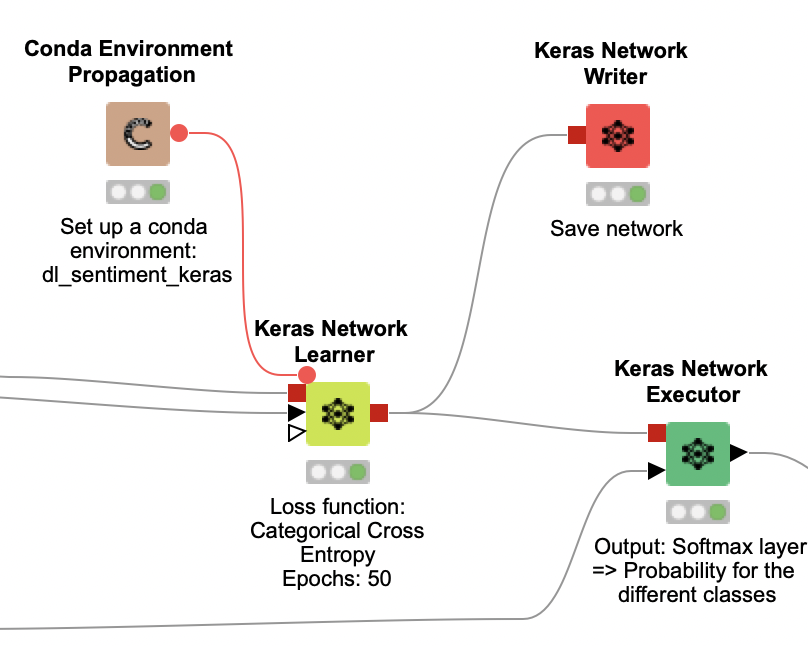
In the Target Data tab, we also have to choose a loss function. Since this is a multiclass classification problem, we use the loss function “Categorical Cross Entropy”.
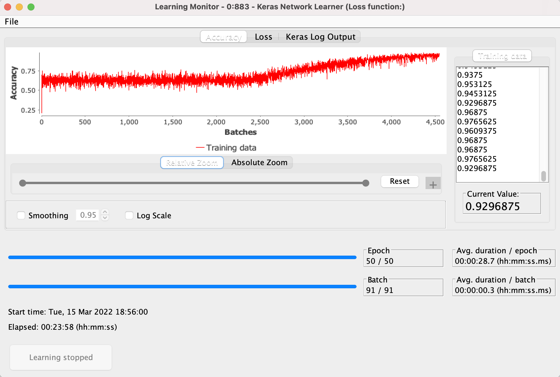
In the Options tab, we can define our training parameters, such as the number of epochs for training, the training batch size, and the option to shuffle data before each epoch. For our application, 50 epochs, a training batch size of 128, and the shuffling option led to a good performance.
Read more about this one-hot vectors for conversion and how to train parameters in text generation with LSTMs.
The Keras Network Learner node also has an interactive view that shows you how the learning evolves over the epochs – that is, how the loss function values drop and how the accuracy increases over time. If you are satisfied with the performance of your training before it reaches its end, you can click the “Stop Learning” button.
We set the Python environment for the Keras Network Learner node, and for the nodes downstream, with the Conda Environment Propagation node. This is a great way of encapsulating all the Python dependencies for this workflow, making it very portable. Alternatively, you can set up your Python integration to use a Conda environment with all the packages listed here.
After the training is complete, we save the generated model with the Keras Network Writer node. In parallel, we use the Keras Network Executor node to get the class probabilities for each tweet in the test set. Recall that we obtain class probabilities here because we use softmax as the activation function of our network’s output layer.
We show how to extract class predictions from these probabilities next.
Evaluate the network’s predictions
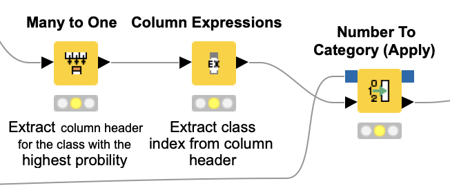
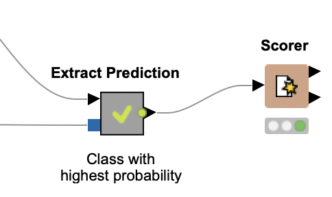
To evaluate how well our LSTM-based predictor works, we must first obtain actual predictions from our class probabilities. There are different approaches to this task, and in this application we choose to always predict the class with the highest probability. We do so because this approach is easy to implement and interpret, besides always producing the same results given a certain class probability distribution.
The class extraction takes place in the Extract Prediction metanode. First, the Many to One node is used to generate a column that contains the class names with the highest probabilities for each test tweet. We post-process the class names a bit with the Column Expressions node, and then map the class indices into positive, negative, or neutral using the encoding model we built in the preprocessing part of the workflow.
With the predicted classes at hand, we use the Scorer node to compare them against the annotated labels (gold data) in each tweet. It turns out that the accuracy of this approach is slightly above 74%: significantly better than what we obtained with a lexicon-based approach.
Note that our accuracy value, here 74%, can change from one execution to another because the data partitioning uses stratified random sampling.
Interestingly, the isolated performance for negative tweets – which correspond to 63% of the test data – was much better than that (F1-score of 85%). Our predictor learned very discernible and generalizable patterns for negative tweets during training. However, patterns for neutral and positive tweets were not as clear, leading to an imbalance in performance for these classes (F1-scores of 46% and 61%, respectively). Perhaps if we had more training data for classes neutral and positive, or if their sentiment patterns were as clear as those in negative tweets, we would obtain a better overall performance.
Deploy and visualize an LSTM-based predictor
After evaluating our predictor over some annotated test data, we implemented a second workflow to show how our LSTM-based model could be deployed on unlabeled data.
First, this deployment workflow re-uses the Tweet Extraction component introduced in our article on lexicon-based sentiment analysis. This component enables users to enter their Twitter credentials and specify a search query. The component in turn connects with the Twitter API, which returns the tweets from last week, along with data about the tweet, the author, the time of tweeting, the author’s profile image, the number of followers, and the tweet ID.
The next step is to read the dictionary created in the training workflow and use it to encode the words in the newly extracted tweets. The "Index Encoding Based on Dictionary" metanode breaks the tweets into words and performs the encoding.
In parallel, we again set up a Python environment with the Conda Environment Propagation node, and connect it to the Keras Network Reader node to read the model created in the training workflow. This model is then fed into the Keras Network Executor node along with the encoded tweets, so that sentiment predictions can be generated for them.
We then read the encoding for sentiment classes created in the training workflow and send both encoding and predictions to the Extract Prediction metanode. Similar to what occurs in the training workflow, this metanode predicts the class with the highest probability for each tweet.
Here we do not have annotations or labels for the tweets: we are extracting them on-the-fly using the Twitter API. For this reason, we can only verify how well our predictor is doing subjectively.
To help us in this task, we implement a dashboard that is very similar to the one in our lexicon-based sentiment analysis project. It combines (1) the extracted tweets; (2) a word cloud in which the tweets appear with sizes that correspond to their frequency; and (3) a bar chart with the number of tweets per sentiment per date.
In terms of structure, we use the Joiner node to combine the tweets’ content and their predicted sentiments with some of their additional fields – including profile images. Next, we send this information to the Visualization component, which implements the dashboard.
Note. This component is almost identical to the visualization one discussed in our lexicon-based sentiment analysis post. Both components just differ a bit in how they process words and sentiments for the tag cloud, since they receive slightly different inputs.
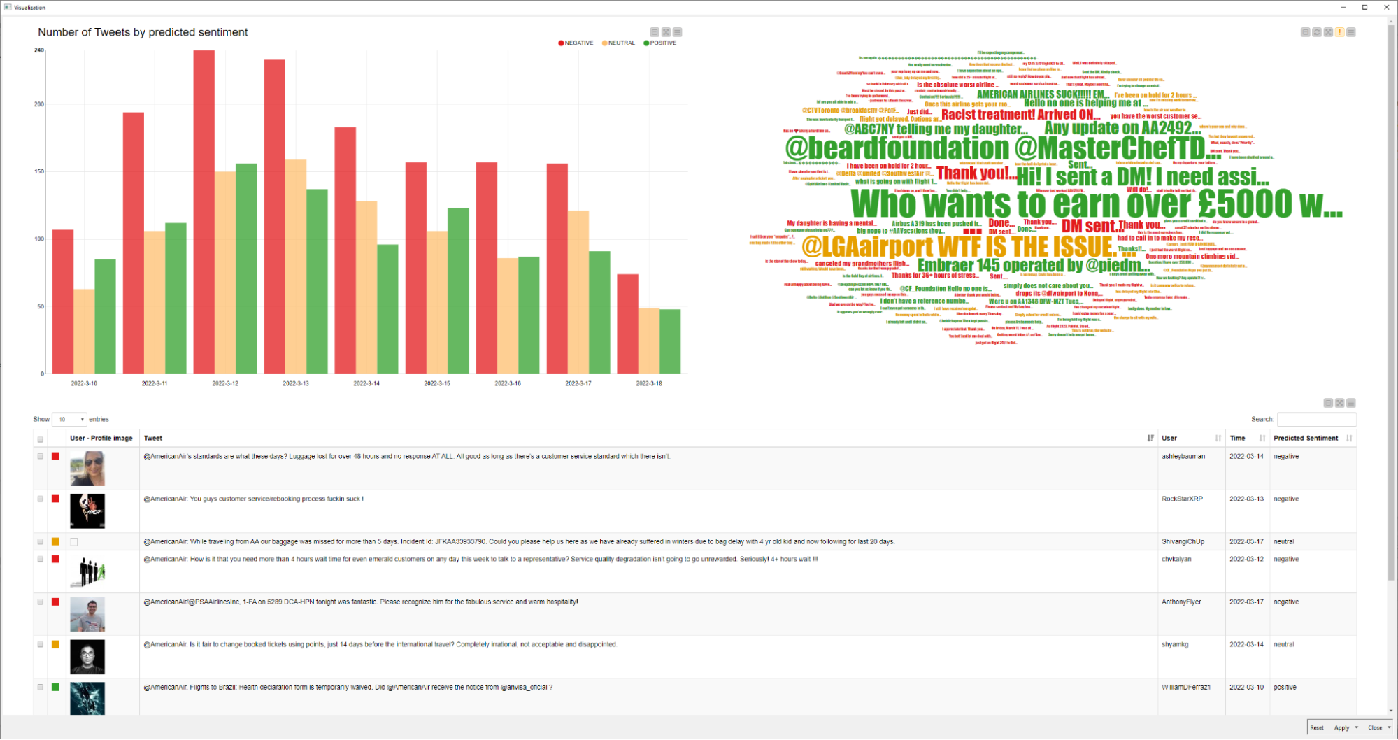
A quick inspection of the tweets’ content in the dashboard also suggests that our predictor is relatively good at identifying negative tweets. An example is the following tweet, which is clearly a complaint and got correctly classified (negative):
"@AmericanAir’s standards are what these days? Luggage lost for over 48 hours and no response AT ALL. All good as long as there’s a customer service standard which there isn’t."
This is aligned with the performance metrics we calculated in the training workflow.
The bar chart also suggests that most tweets correspond to negative comments or reviews. Although it is hard to verify if this is really the case, this distribution of sentiment is compatible with the one in the Kaggle dataset we used to create our model. In other words, this adds to the hypothesis that airline reviews on Twitter tend to be negative.
Finally, the tweets in Figure 8 give us an opportunity to discuss a limitation of our sentiment analysis. The most common tweet, which is the largest one in the tag cloud, is a likely scammy spam that got classified as positive:
"@AmericanAir Who wants to earn over £5000 weekly from bitcoin mining? You can do it all by yourself right from the comfort of your home without stress. For more information WhatsApp +447516977835."
Although this tweet addresses an American airline company, it does not correspond to a review. This is indicative of how hard it is to isolate high quality data for a task through simple Twitter API queries.
Note that our model did capture the positivity of the tweet: after all, it offers an “interesting opportunity” to make money in a comfortable and stress-free (many positive and pleasant words). However, this positivity is not of the type we see in good reviews of products or companies — human brains quickly understand that this tweet is too forcedly positive, and likely fake. Our model would need much improvement to discern these linguistic nuances.
LSTM-based Predictor: Better for negative tweets
LSTM-based sentiment analysis is relatively simple to implement and deploy with KNIME. The predictor we discuss in this article performs significantly better than a lexicon-based one, especially for negative reviews. This probably happens because (1) the training data for the model contains many more negative reviews, biasing the learning; and (2) the language patterns in negative reviews are clearer and thus easier to be learned. To an extent, we could improve the performance of our predictor by improving the quality and amount of training data.
Adding a dashboard to the deployment workflow was once again useful. Through visualizations and at a low cost, we could gather insights on how our predictor works for unlabeled tweets, and even detect a potential data quality issue with spams. This is exactly the type of resource that saves data analysts a lot of time in the long run.
Note: Explore the workflows used in this article, showing how to build and deploy LSTM-based sentiment predictors.
References
F. Villaroel Ordenes & R. Silipo, “Machine learning for marketing on the KNIME Hub: The development of a live repository for marketing applications”, Journal of Business Research 137(1):393-410, DOI: 10.1016/j.jbusres.2021.08.036.