“Once Upon A Time … “ by LSTM Network

Recurrent Neural Networks (RNN) are the state of the art for sequence analysis ^{5 6}. With the release of KNIME Analytics Platform 3.6, KNIME extended its set of deep learning integrations, adding the Keras integration to the DL4J Integration. This adds considerably more flexibility and advanced layers, like RNN Layers.

In this article, we want to find out what Recurrent Neural Networks are in general, and LSTMs in particular. Let’s see where they are useful and how to set up and use the Keras integration in KNIME Analytics Platform to implement them.

As a use case for this particular application of RNNs and LSTMs we want to focus on automatic text generation. The question is: Can we teach KNIME to write a fairy tale?

Recurrent Neural Networks are a family of neural networks used to process sequential data. Recently, they have shown great success in tasks involving machine translation, text analysis, speech recognition, time series analysis, and other sequence-based problems^{5 6}.

RNNs have the advantage that they generalize across sequences rather than learn individual patterns. They do this by capturing the dynamics of a sequence through loop connections and shared parameters ^{2 6}. RNNs are also not constrained to a fixed sequence size and, in theory, can take all previous steps of the sequence into account. This makes them very suitable for analysing sequential data.

Technically RNNs can be seen as a chain of multiple copies of the same static network A, with each copy working on a single time step of the input sequence. The network copies are connected via their hidden state(s). This means that each of the network copies has multiple inputs: the current value $x(t)$ and the hidden state(s) $h(t-1)$ as the output from the previous copy.

A common way of depicting an RNN with a loop connection is shown on the left in Figure 1. The network A (green box) is a static network with one or multiple layers. The loop connection indicates that the output of network A at one time step $t$ is used as the input for the next time step $t + 1$.

On the right in Figure 1 we see the unrolled graph of the same network, with multiple copies of network A. Note that “a copy of network A” here really indicates the same weights and not just the same network structure. To train RNNs a generalized Back Propagation algorithm is used, which is known as Back Propagation Through Time (BPTT) ².

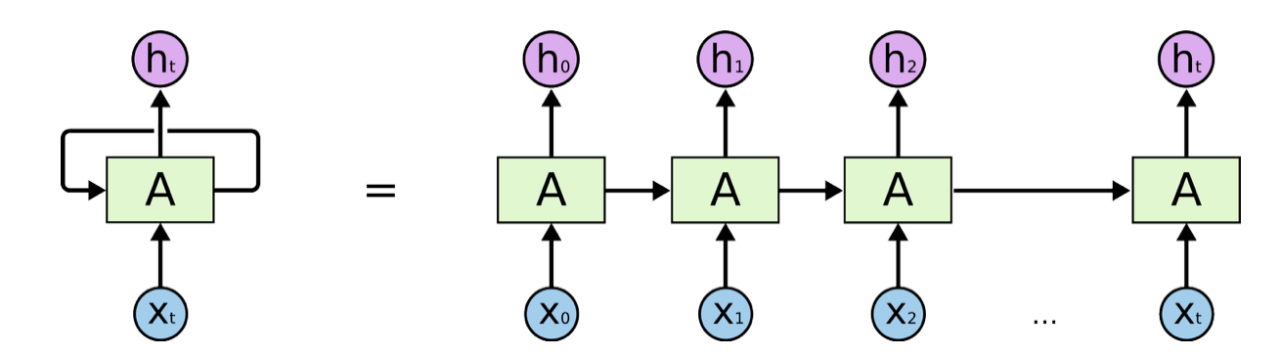
Figure 1. A Recurrent Neural Network (RNN) is a network A with recurring (looping) connections, depicted on the left. The same RNN is represented on the right as a series of multiple copies of the same network A acting at different times t. Image reproduced from ¹.

While RNNs seemed promising to learn time evolution in time series, they soon showed their limitations in long memory capability. This is when LSTM (Long Short Term Memory) sparked the interest of the deep learning community ³.

An LSTM network is a special type of RNN. Indeed, LSTM networks follow the same chain-like structure of network copies as RNNs. The only difference is in the structure of network A.

To overcome the problem of limited long memory capability, LSTM units use the concept of an additional hidden state to $h(t)$: the cell state $C(t)$. $C(t)$ represents the network memory. A particular structure, called gates, allows you to remove (forget) or add (remember) information to the cell state $C(t)$ at each time step based on the input values $x(t)$ and hidden state $h(t - 1)$ (Figure 2).

Each gate is implemented via a sigmoid layer that decides which information to add or delete by outputting values between 0 and 1. By multiplying the gate output pointwise by a state, e.g. the cell state $C(t-1)$, information is deleted (output of gate ≈ 0) or kept (output of gate ≈ 1).

In Figure 2, we see the network structure of an LSTM unit. Each LSTM unit has 3 gates. The “forget gate layer” at the beginning filters the information to throw away or to keep from the previous cell state $C(t - 1)$ based on the current input $x(t)$ and the previous cell’s hidden state $h(t - 1)$.

The adding of information to the cell state $C(t)$ consists of two layers: An “input gate layer” that decides which information we want to add and a “tanh layer” that forces the output between and -1 and 1. The outputs of the two layers are multiplied pointwise and added to the previous, already filtered cell state $C(t - 1)$ to update it.

The last gate is the “output gate”. This decides which of the information from the updated cell state $C(t)$ ends up in the next hidden state $h(t)$. Therefore, the hidden state $h(t)$ is a filtered version of the cell state $C(t)$.

For more details about LSTM units, check the Github blog post “Understanding LSTM Networks” (2015) by Christopher Olah.

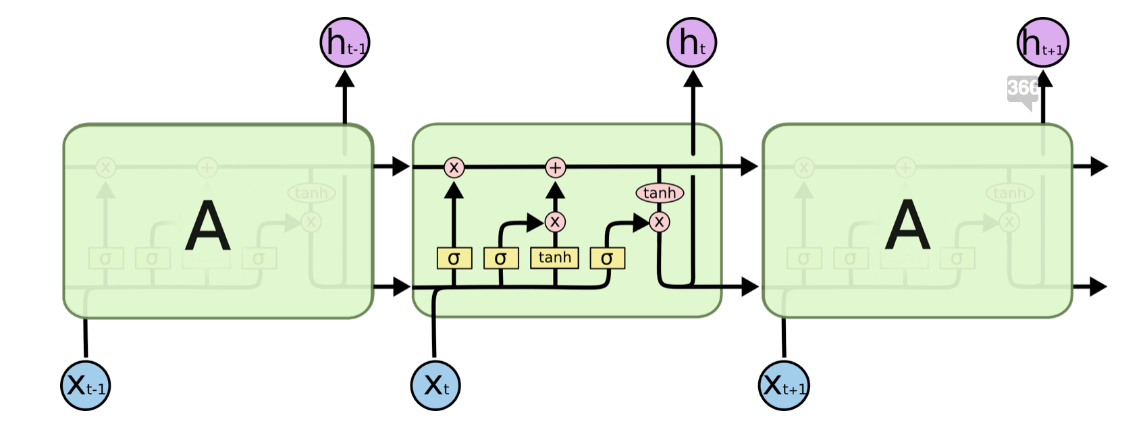
Figure 2. Structure of an LSTM cell (reproduced from ¹). Notice the 3 gates within the LSTM units. From left to right: the forget gate, the input gate, and the output gate.

For different tasks a different input to output mapping is required ^{6 7}. For example, many-to-many for translation, many-to-one for sentiment analysis and one-to-many for image captioning ⁷.

To face the different possible input to output mappings, the Keras LSTM Layer node in KNIME Analytics Platform gives you the option to either return only the last state for a many-to-one model, or to output the whole sequence for a many-to-many model.

In addition, in order to use the content state $C(t)$, e.g. in machine translation, you can activate the checkbox, Return state, in the configuration window.

Many people love Grimm’s fairy tales. Unfortunately, the Grimm brothers are not alive anymore to write new fairy tales. But maybe we can teach a network to write new stories in the same style? We trained an LSTM many-to-one network to generate text at character level using the Grimm’s fairy tales as training material. The new fairy tale, LSTM generated, starts as follows:

“There was once a poor widow who lived in a lonely cottage. In front of the cottakes, who was to sleep, thit there was not one to sing, or looked at the princess. ‘Oh, what should reached now?’ said the truth; and there they sounded their protistyer-stones. Then they were stronger, so that they should now look on the streets, not rolling one of them, for the spot were to rung”

The network really has learned the structure of the English language. Although it’s not perfect you can see common character combinations, words, usage of quotation marks, and so on.

To reach this result, we needed to prepare the text and the network going through a number of different steps. These steps are pre-processing, encoding, defining, and training a many-to-one LSTM network, and finally a deployment workflow to apply the trained network.

This same network with the same pre-processing steps could be retrained on different languages and texts in order to create new texts in different languages and speaking styles.

We will start to train our network by using a subset of Grimm’s fairy tales, which we downloaded from the Gutenberg project.

For the training, we used semi-overlapping sequences of the same length where each character is encoded by an index. To make this clearer, let’s take a look at an example using the following sentence:

“KNIME Analytics Platform has a Keras integration”.

On the left side of Figure 3 we see the semi-overlapping sequences using an arbitrary length of 10 characters. When the network gets the input sequence “KNIME Anal” we want it to predict that the next letter will be “y”. When it sees “NIME Analy” the output should be “t” and so on.

In addition, we need to encode each character with an index. Therefore, we created and applied a dictionary to end up with what you can see on the right in Figure 3.

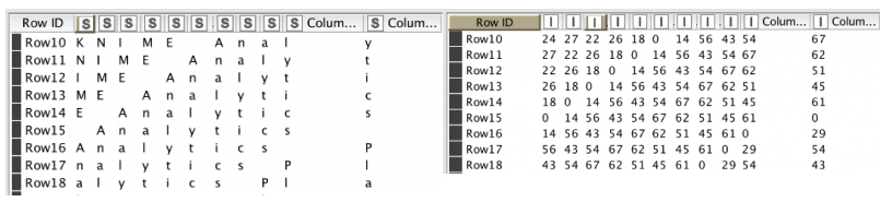
Figure 3. For the training we use semi overlapping sequences. On the left side we see the sequences still using characters. On the right we the sequence after applying a dictionary.

In Figure 4 we see the training workflow, including the part that actually performs the pre-processing and encoding task. The general idea is that we separate each character and represent the whole text in one column and one character per row. The reshaping is done to avoid a loop to apply the dictionary to speed up execution. Next, we apply a dictionary and create our semi-overlapping sequences. Here are the steps:

1. Reshape the text into one column of characters
2. Create a character dictionary
3. Use the Cell Replacer node to apply the dictionary
4. Create the overlapping sequences of length 100 using the Lag Column node
5. Resort the columns
6. Create the collection columns for the input and the target

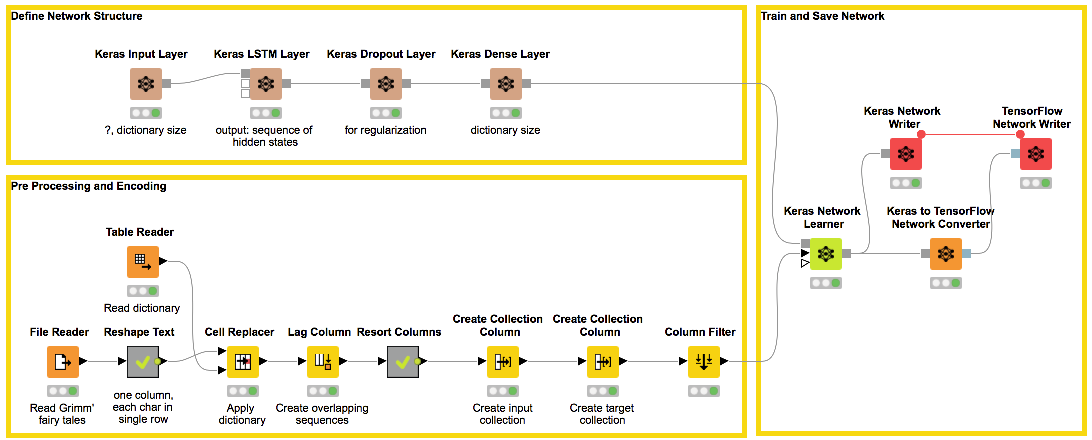
Figure 4. This workflow uses Grimm’s fairy tales to train an LSTM network to generate text in fairy tale style. The Pre-processing and Encoding part reads Grimm’s fairy tales and creates the semi-overlapping sequences used to train the network. The brown nodes defines the network structure and the Keras Network Learner node trains the model using TensorFlow in the backend. For faster prediction in the deployment workflow the Keras model is converted into a TensorFlow model and saved.

Figure 5 shows you what happens inside the “Reshape Text” metanode.

We go through the following steps to reshape the text:

1. The String Manipulation node replaces any character with the character plus a space
2. The Cell Splitter node splits the text on every space
3. The Constant Value Column node adds a space at the end of each line
4. The Unpivoting node puts the whole text in one column
5. The Row Filter node deletes missing values

In addition, we also create and write our dictionary. Therefore, we first delete duplicate characters with the GroupBy node, before we use the Counter Generation node to assign the index to each character.

Figure 5. This is the inside of the Reshaping Text metanode. The workflow snippet transforms the full text into one column, one character per row. In addition it creates a dictionary for the encoding.

Before we can use the Keras Network Learner node to train the network we need to define its structure. Looking at the workflow in Figure 4, the brown nodes define the network structure.

• The Keras Input Layer node requires the input shape of our network. In our case this is a 2^nd order tensor. The first dimension is the sequence length. The second dimension the dictionary size, as the network works on a one-hot-vector representation of our sequence of indices. We will allow variable input length and our dictionary has 73 different characters. Therefore the input shape is “?, 73”.
• The Keras LSTM Layer node has two optional input ports for the hidden states, which we can define further in the configuration window. For our model, we choose to use 512 units, which is the size of the hidden state vectors and we don’t activate the check boxes, Return State and Return Sequences, as we don’t need the sequence or the cell state.
• The Keras Dropout Layer node is used for regularization.
• The Keras Dense Layer node defines the final activation function for the output. In our case this is softmax, which will output the probability for each character in our dictionary. Therefore, we set the number of units to the number of different characters in our dictionary. In our case 73.

Now we have our network as well as the preprocessed and encoded data, so we are nearly ready to train our network. Last, we have to set the training settings in the configuration window of the Keras Network Learner node.

The Keras Network Learner node has three input ports: A model port for the network, a data port for the training data, and an optional port for the validation set.

The Keras Network Learner node has four tabs. We will focus now only on the first 3: The Input Data, the Target Data, and the Options tab.

In the Input Data tab we select From Collection of Number (integer) to One-Hot-Tensor to handle conversion and select the collection with our input sequence. We need this conversion because our network doesn’t learn directly on the sequence of integers, but on a sequence of one-hot-vectors. In the Target Data tab we select From Collection of Number (integer) to One-Hot-Tensor again and choose our collection with the target value. Next, we have to choose a loss function. Here we can choose between a standard loss function and defining an own custom loss function. As this is a multiclass classification problem we use the loss function, “Categorical Cross Entropy”.

In the Options tab we can define our training parameters, e.g. the back end, how many epochs we want to train, the training batch size, the option to shuffle training data before each epoch and the optimizer with its own parameters.

For training, we use 50 epochs, a training batch size of 512, the shuffling option and as optimizer Adam with default settings for the learning rate. The blog post “An overview of gradient descent optimization algorithms” gives you an overview of the different types of gradient descent optimization.

In Figure 6 you can see the view of the Keras Network Learner node. It shows you how the accuracy changes over the epochs. Click the Stop learning button to stop learning once you are satisfied with the reached accuracy.

The Keras Network Writer node saves the trained model. In addition, we converted it into a TensorFlow Network using the Keras to TensorFlow Network Converter node. We use the TensorFlow network in our deployment workflow because it avoids a time-consuming Python startup, which would be necessary if we used the Keras network.

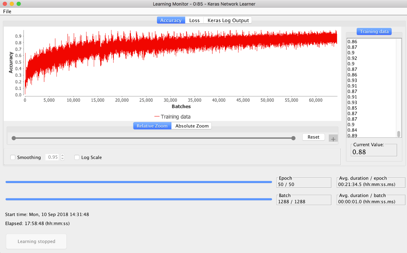
Figure 6. The view of the Keras Network Learner node. It shows how accuracy changes during training.

To execute the network, we start with an input sequence of the same length as each of the training sequences. Then we apply our network to predict the next character, delete the first character, and apply the network again to our new sequence and so on.

To do this in KNIME Analytics Platform we can use a recursive loop.

To create a recursive loop we need the Recursive Loop Start and End node. The input of the Recursive Loop Start node is only used in the first iteration. For the following iterations, the input of the second input port of the Recursive Loop End node is used as loop input. The first input port of the Recursive Loop End node expects the data that will be collected across the iterations.

In our case this means that we want to feed into the second input port a collection of the same length as the input where the first character of the sequence of the previous iteration is deleted and the predicted character is added. The first input port is simply given the predicted character.

Figure 7. This is the deployment workflow. It reads the beginning of a fairy tale and our trained network. Then it predicts one character after the other.

Figure 7 shows the deployment workflow. In the Extract Index metanode we use the probability distribution over all possible indexes to make the predictions. Here we have two options. We can either always predict the index with the highest probability or we can pick the next index based on the given probability distribution.

Both techniques are possible in KNIME Analytics Platform with either the Many to One node (Figure 8) or the Random Label Assigner (Data) (Figure 9).

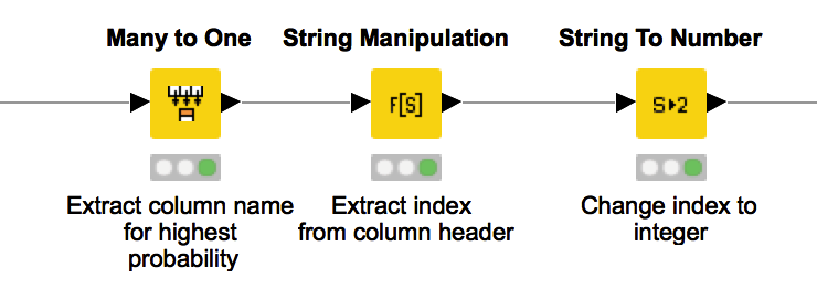
Figure 8. This workflow snippet takes as input the output probability distribution of the executed network and extract the index with highest probability.

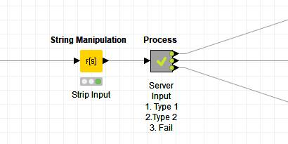
Figure 9. This workflow snippet expects as input the probability distribution for the different indexes and picks one according to it.

The many to one approach is easier to implement. It has the disadvantage that the network is deterministic and will always produce the same results. The second approach leads to a model that is not deterministic, as we pick the next character according to a distribution, and therefore leads to different results whenever we execute the loop.

• Download the Generate Fairy Tales workflows from the KNIME Hub here.

By changing the input file you can train a network that generates text in the style and language you want.

The KNIME Deep Learning Extension integrates deep learning functionalities from Keras via Python. For the training you can choose between TensorFlow, CNTK and Theano as backend.

Without writing a single line of code, this integration allows you to:

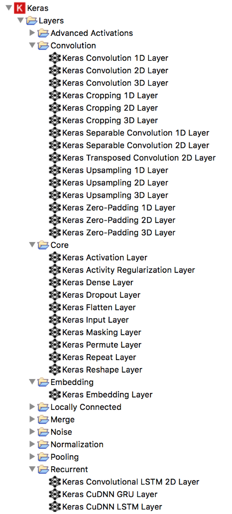
- build your own network structure using the more than 60 different layer nodes

- train your own network from scratch with the Keras Network Trainer node

- execute trained networks

- read pre-trained Keras networks for transfer learning

- execute trained network

If you prefer to write code, KNIME has also a Python Deep Learning integration, which you can mix and match with the Keras integration, for example to edit trained networks.

Last but not least, the TensorFlow Integration allows you to convert a Keras network into a TensorFlow model.

You can see that this integration gives you a lot of functionality!

The nodes in this extension rely on a Python installation with Keras and TensorFlow. In case you have a GPU available you can install and use the keras-gpu library to accelerate training.

In summary, to run Deep Learning and Keras nodes in KNIME Analytics Platform, you need to:

• install Python with Keras and TensorFlow on your machine
• install the KNIME Python Integration and KNIME Deep Learning – Keras Integration Extensions in KNIME Analytics Platform
• set default Python and Keras path in KNIME Analytics Platform preferences

Note. Installation details are available in the KNIME Deep Learning Extension - Keras Integration web page. Please follow them thoroughly.

---

[1] “Understanding LSTM Networks” (2015)

[2] Ian Goodfellow, Yoshua Bengio and Aaron Courville, “Deep Learning”, The MIT Press, 2016

[3] Hochreiter & Schmidhuber (1997)

[4] https://en.wikipedia.org/wiki/Recurrent_neural_network

[5] Crash Course in Recurrent Neural Networks for Deep Learning

[6] A Critical Review of Recurrent Neural Networks for Sequence Learning

[7] The Unreasonable Effectiveness of Recurrent Neural Networks