
Many tools and techniques for data science are moving ahead at an astronomical speed. Deep learning is one such technique, leveraged to attain groundbreaking results.
Deep-learning-based predictive models are used in various sensitive applications across banking, medical systems, and criminal justice. Building these complex applications has become easier thanks to codeless tools.
These applications sound interesting, but what if some of your application users or fellow team members ask you a specific question about how they work, like “Why is this instance predicted with a negative outcome?” or “Can you explain the predictions of the AI model you trained?” In moments like this, you realize such an application is merely a black box.
What is XAI?
Explainable AI (XAI) is the set of techniques used to interpret the behavior of black box models. Techniques in XAI can be divided into two categories: global and local explanations. Global explanation concerns the behavior of the black box on an overall level. For example, global feature importance is a global technique denoting how important a particular feature is for the model’s outcome in all the instances. Local explanations deal on a single instance level. For example, a local explanation can point out which features contributed most to the outcome of a single prediction.
What are Counterfactual Explanations in XAI?
A Counterfactual Explanation is an XAI technique used to generate local explanations. Imagine a black-box model that classifies whether a loan application should be accepted or rejected based on three features of an applicant: “age,” “number of debts,” and “income.” If the outcome for a particular user profile is “loan application rejected” its counterfactual instance would be “loan application approved.” We can explain the outcome “loan application rejected” by computing the minimal changes that could be made to the instance feature values so that the black box alters the prediction to its counterfactual (“loan application approved”) (Fig. 1).
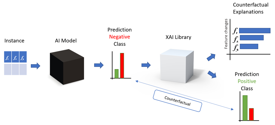
So the counterfactual explanation consists of a list of feature changes. In our loan approval example, we could produce this counterfactual explanation: “The loan was rejected because the applicant is 10 years too young and his yearly income is USD 10,000 too low.” This same explanation could be represented by the vector “(Age: +10, Number of debts: 0, Income: +10k).”
Counterfactual explanations are intuitive, and provide reasoning to users on what changes are required from their end. This reasoning can be easily comprehended by humans, thereby making the black box interpretable to a certain extent.
How Do You Find Counterfactual Instances?
Finding a counterfactual instance means computing the feature changes needed to go from the original feature values in an instance with vector X to a new vector X’, which leads to the opposite model outcome (the counterfactual). Keep in mind that X and X’ can be represented as vectors in a feature space of n dimensions, where n is the number of input features in our model. The model builds a curve (decision boundary) in the feature space that divides it into different areas based on the outcome.
To demonstrate how a counterfactual is represented in the feature space, let’s make a simple example with a model with only two features (Fig. 2). This space is two-dimensional, with Feature 1 on the y-axis and Feature 2 on the x-axis. The blue area represents the positive class, while the white area represents the negative class. Consider the given instance as X in the blue area; we want to find the counterfactual for this instance.
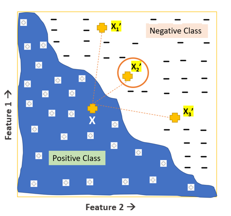
There are two basic conditions for finding a human-interpretable counterfactual X’ for the given instance X:
-
Condition 1: The predicted class of the model for X’ should be different from X.
-
Condition 2: The distance between X and X’ should be minimal.
The first condition is about getting a different predicted class, while the second is a constraint that tries to minimize the distance between these instances. When X and X’ are close, it means that only a few features and small values are changed, making the changes intuitive and meaningful for humans.
As shown in Fig. 2, X’2 is the optimal counterfactual for the given instance X. With this two-dimensional feature space, it was easy to visually locate the optimal counterfactual. In order to find counterfactual explanations in an n-dimensional feature space, we need to apply the following algorithm.
We can search for X′ using a simple optimization problem with the following function (Fig, 3):
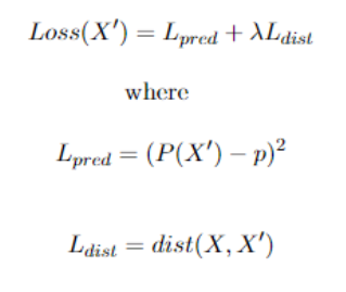
The first term Lpred ensures that the counterfactual instance prediction P(X’) is as close as possible to the counterfactual outcome, p, a parameter to be defined beforehand based on Condition 1. The second term Ldist requires the Manhattan Distance between the two instances X and X’ to be as small as possible (Condition 2).
At times X’ is discarded, as its predicted class is not the counterfactual class. The parameter 0
This technique is implemented in the Python package alibi. After defining a few parameters, the python library provides a function that takes as input the black-box model and the instance X. The python package finds for us the optimal counterfactual instance X’, from which we can find the counterfactual explanation for the prediction of X with a simple difference.
How Do You Find Counterfactual Instances Using KNIME?
The KNIME Python Integration allows us to smoothly integrate Python code inside KNIME workflows. What's more, we can wrap this code into reusable components that can be shared and used as KNIME nodes and utilize the power of Python libraries. Based on this, we have created the KNIME component Counterfactual Explanations (Python).
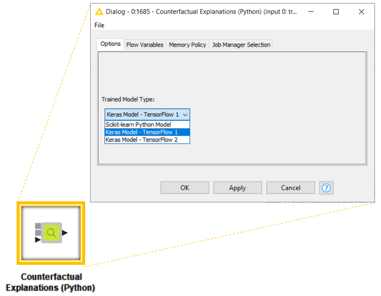
This component generates intuitive and local explanations for each prediction from a binary classification model trained either using the KNIME Deep Learning – Keras Integration or the KNIME Python Integration via Scikit-learn. In the configuration panel, the user can select the model type beforehand. To compute the explanation, any adopted Python package (alibi, keras, scikit-learn, etc.) is automatically installed via a Conda Propagation node if one is not already available.
The component and its configuration panel are shown in Fig. 4. The component has three input ports:
-
Port 0: Trained model from Keras Network Learner, Python Learner, or Python Object Reader
-
Port 1: Pre-Processing Pickled Object from Python Object Reader or Data Preprocessing for Keras Model component.
-
Port 2: Row instances to be explained. Those rows should be in raw format — not normalized before the preprocessing Python script was applied.
Demonstration of Counterfactual Explanations (Python) component based on use case
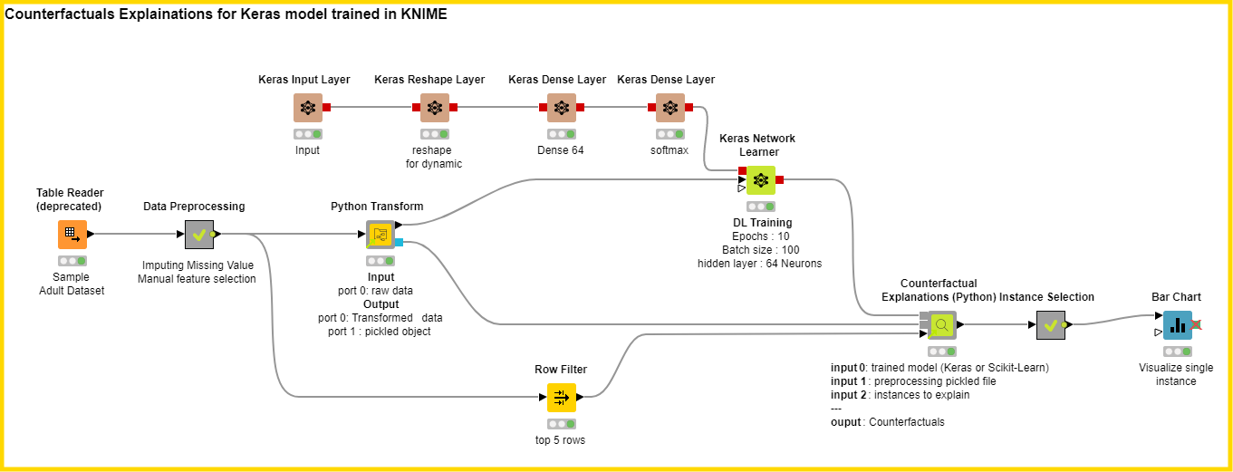
Let's explore a use case to understand this component. The example workflow is shown in Fig. 5. We have considered the publicly available adult income dataset for binary classification. The objective is to identify whether a person’s income is higher or lower than USD 50,000, based on the personal characteristics available in the data set.
First we import the data to KNIME Analytics Platform. Next we perform the data transformation tasks using the Python Transform' component so that we can capture the process in a pickled file. To learn more about how this component works, read our blog post Share Python Scripts in Components: Faster Collaboration. The transformation has to be captured in a pickled file so that the component can preprocess the supplied instances and then compute the counterfactual instances. Then we train a simple Keras model to carry out the task of classification. This model can be now used to predict someone’s income based on their personal characteristics.
Now we want to explain the Keras model for some particular instances of interest using the counterfactual explanations. We select five instances in which the income prediction is less than USD 50,000. We want to find out what minimal changes in these people's characteristics would make the model predict their income as higher than USD 50,000.
We connect the trained Keras model to the first input port (Port 0) and the preprocessing pickled file to the second input port (Port 1). Finally we supply these instances to the Counterfactual Explanations (Python) component. In the configuration panel we select “Keras Model - TensorFlow 1” as a trained model type, as required by the KNIME Deep Learning – Keras Integration.
The component outputs the results in a single table (Fig. 6), where each row represents a counterfactual explanation:
-
The predicted class for the original instance X in the column “Prediction”
-
The predicted class for the counterfactual instance X’ in the column “Counterfactual”
-
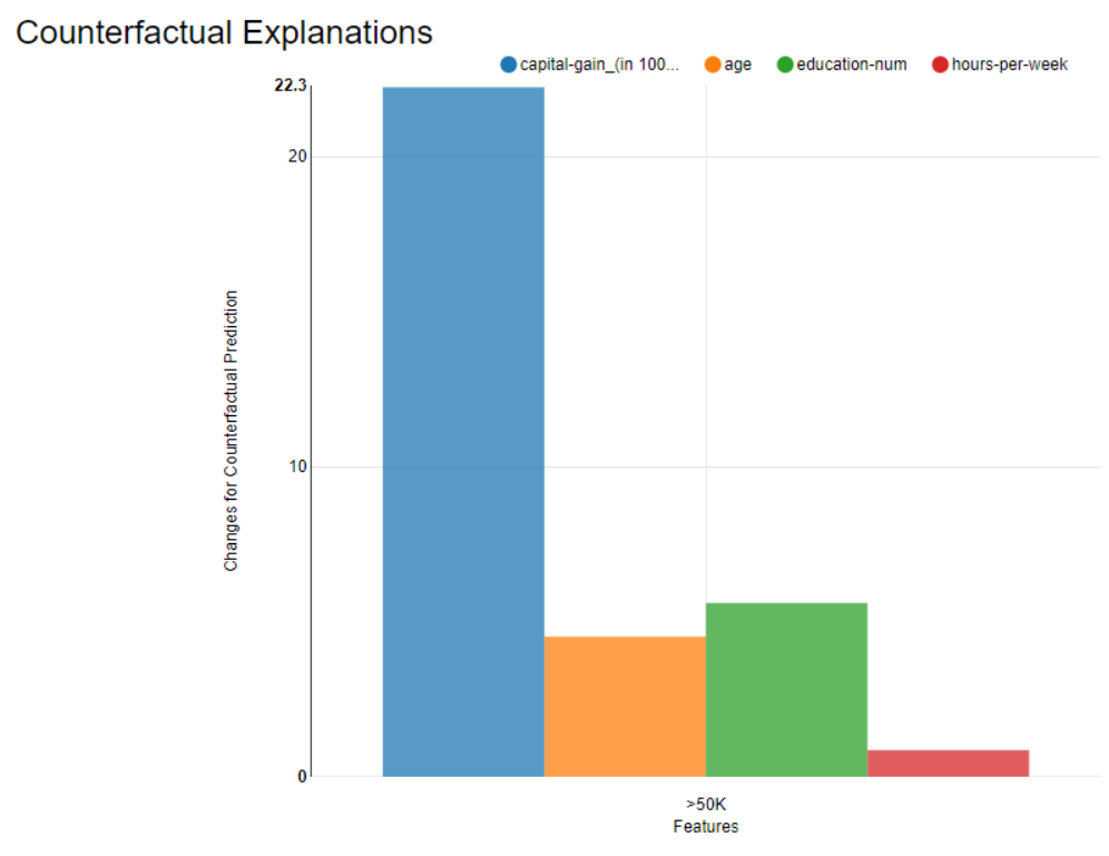
The explanation, represented as a list of feature changes required to go from X to X’
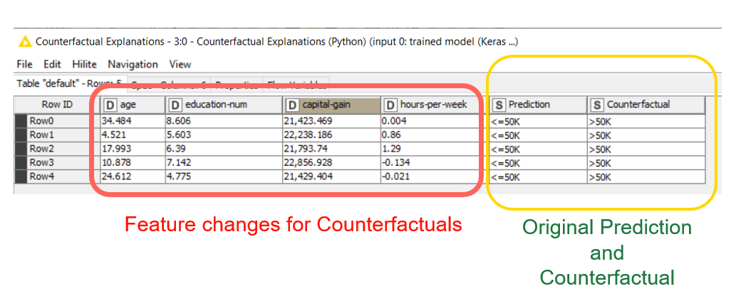
The subject in Row 1 in Fig. 6 was predicted by the model as low income (“
More Codeless XAI Components to Understand Black-Box Models
In this post, we highlighted the importance of understanding black box models, then specifically focused on counterfactual explanations, which constitute one of the XAI techniques for local explanations. Next we briefly looked at the mathematical method for finding counterfactual explanations implemented in a Python library “alibi.”
We then showed the KNIME component “Counterfactual Explanations (Python),” which adopts the same library, and a workflow, Train and Explain Keras Network with Counterfactuals, showing how to use the component to explain a Keras deep learning model trained in KNIME Analytics Platform. To explore more workflows containing this component, visit this dedicated KNIME Hub space.
The Counterfactual Explanations (Python) component is a part of the Verified Components project, where many other components are built, reviewed, and shared by the KNIME team. Other verified components for XAI use cases are described in the blog post How Banks Can Use Explainable AI (XAI) For More Transparent Credit Scoring.