Time Series Temperature Prediction from IoT Sensor Data

Across industries, companies are losing money due to waste, be that wasteful energy management or poor use of capacities or assets. IoT prediction initiatives can play a key role here to enable companies to plan and operate more efficiently. IoT-based temperature prediction is already being used successfully by manufacturers to manage their energy consumption more efficiently or by farmers to evaluate weather information in order to predict potential crop yields more efficiently.

In this article we want to look particularly at time series analysis for IoT. Time series data is typical for sensor data from smart electricity meters or in meteorology for forecasting the weather. Data collection from IoT sensors and its storage can be quite a challenge, considering its high volume. Today, however, we want to look at how, after collecting the data, we can analyze it to make predictions.

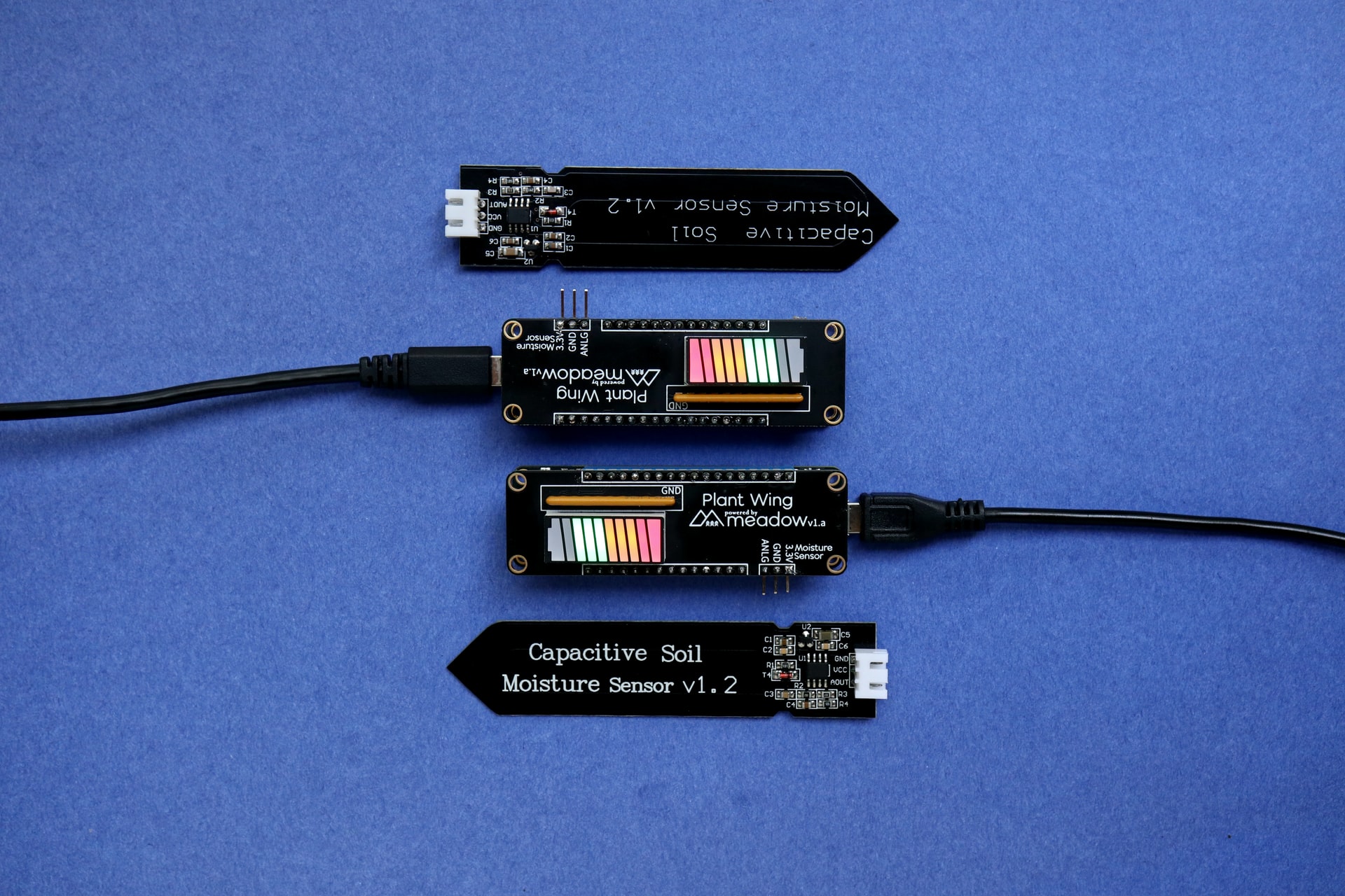
This article is based on a solution we built with KNIME software to forecast temperature. To recap, we collected our data using a sensor board by Arduino, set up a Snowflake database for data storage, and transferred the data from the sensor board to Snowflake via a REST service.

Note. Read more in the article Data Collection from IoT Sensors

Now let’s take our example solution and show how we:

• Trained a sARIMA model to predict the temperature in the next hour

• Developed an application to clean up and process the acquired data and to train the sARIMA model

• Built a dashboard application to predict the next hour temperature using the sARIMA model along with expected minimum and maximum temperature of the following day.

Note. You can find all applications used to build this weather station on the KNIME Hub in KNIME Weather Station

The sensor board was mounted on the outside of a window at our workplace. Readings were received almost once per minute, and data were collected for at least one month, totaling over 30k observations (i.e. data rows).

IoT sensors produce time based signals that can be nicely processed with time series analysis algorithms. Before moving into the training or deployment of the algorithms, it is necessary to clean and standardize the time series. This means:

• Aggregate data into a hourly average
• Perform some Time Alignment as to have value for every hour, adding missing values where needed
• Impute Missing values using Linear Interpolation
• Calculate the Seasonality index
• Visualize the Time Series with a Line Plot node

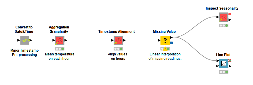
Time Alignment, Aggregation Granularity, and Inspect Seasonality components have been used to implement the part for time alignment, aggregation into an hourly average, and seasonality index calculation, respectively (Fig. 1). These and more components are available in the Time Series Component Extension for performing the basic transformations for time series analysis.

A good overview of our time series components is given in this blog article, Time Series Analysis with Components. Definitely check them out!

Download the workflow KNIME Weather Data Inspection and Visualization from the KNIME Hub to try out for yourself.

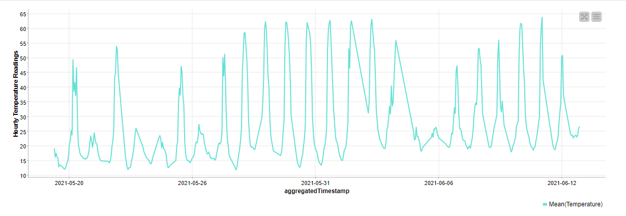
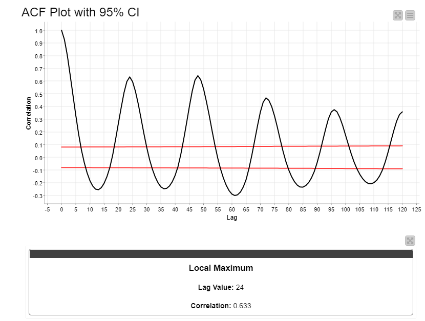
The plot of the temperature time series (Fig. 2) shows cyclic peaks, which indicate observable seasonality. However, seasonality was more precisely inspected, using the Inspect Seasonality component. The Inspect Seasonality component takes the time series at the input port and calculates its Auto-Correlation Function (ACF) over a set time interval (Fig. 3). In our case, on a 120 hours time window, we see a first peak at 24h, then a second peak at 48h, and decreasing peaks at every multiple of 24h. The first local maximum usually indicates a possible seasonality. Repeating peaks at multiples of the first peak position confirm that seasonality, in our case a 24-hour seasonality.

Now let’s train a sARIMA model to forecast the temperature values in the next hours using the temperatures from the past 24 days. sARIMA or (Seasonal)ARIMA is an enhanced version of the ARIMA model that explicitly also models the seasonality within the data. Indeed, sARIMA adds an ARIMA model for seasonality to the classic ARIMA model for the remaining data. The parameters are thus (p, d, q) for the classic ARIMA model and (P, D, Q) for the seasonal ARIMA model dedicated to modeling seasonality.

Thus the sARIMA model seemed to suit this problem well, given the clear 24h seasonality emerged from the ACF plot.

In total, sARIMA requires 7 parameters:

• p and P: indicate the number of autoregressive terms in the two ARIMA models respectively.
• d and D: indicate the number of differences (i.e. the differencing order) applied to the data before the respective ARIMA model is applied.
• q and Q: indicate the number of moving average terms in the two ARIMA models.
• s: indicates the seasonality index in the data (in this case: 24).

Note. Further details of the sARIMA model can be found in the blog article, S.A.R.I.M.A. Seasonal ARIMA Models with KNIME.

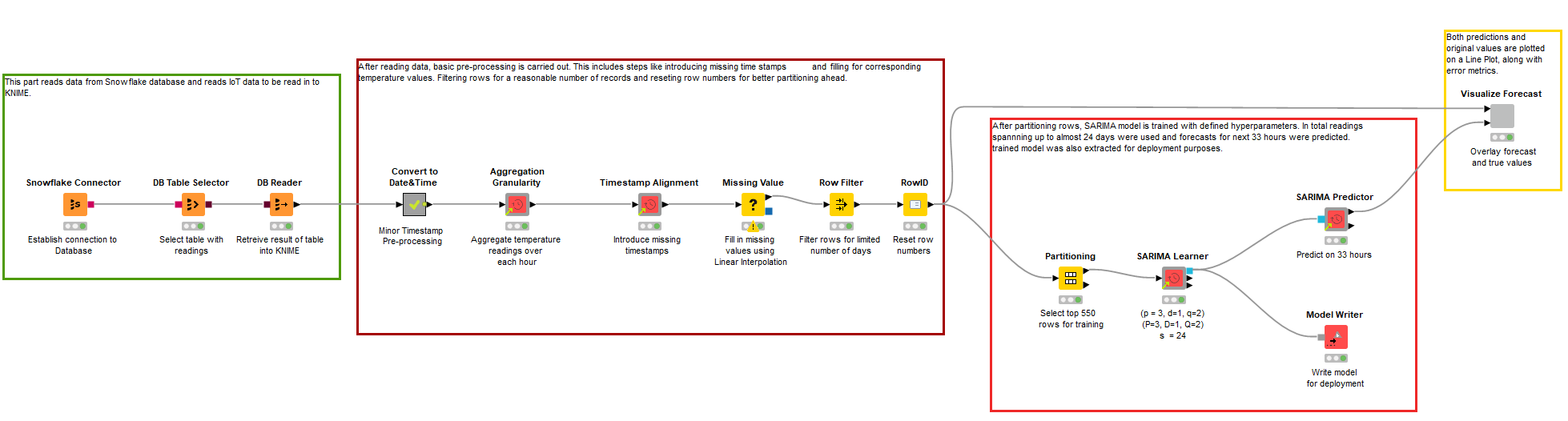
There were 583 rows after aggregation on hourly average of temperature data recordings. Records were then partitioned in such a way that the first 550 rows were used for training the model and the remaining rows for testing it.

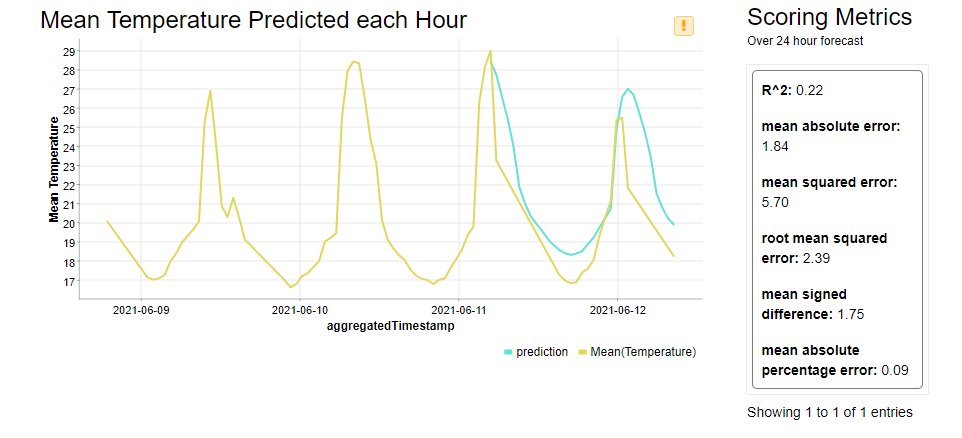
We iterated on a number of different sARIMA models with different sets of hyperparameters (p, d, q) (P, D, Q). The most successful model was (p = 3, d=1, q=2), (P=3, D=1, Q=2) and s = 24. In Fig. 5 we have reported the original temperatures in yellow and the predicted temperatures over the test set in light blue, for the best sARIMA model. Predictions were made from past real values of the test set and plotted along (the remaining 33 rows out of 583). This testing technique produced a MAE (Mean Absolute Error) of 1.84, i.e. on a range of [15, 29] produced a MAPE (Mean Absolute Percentage Error) of 9%, which seemed acceptable.

To learn more about scoring metrics, check the article Numeric Scoring Metrics' on Analytics Vidhya.

Note. The training workflow KNIME Weather Data Cleaning and Model Training can be found on the KNIME Hub.

The last part of this project covers the adoption of the trained sARIMA model in production. The sARIMA model can forecast the temperature for the next few hours. However, knowledge of the next hour’s temperature is of limited usage even in the German summer. What would be more useful for us is to have an idea of tomorrow’s temperatures, so that we can get out of the house in the morning properly dressed to face the weather of the day. So, what about predicting the temperatures for the whole day tomorrow and extracting the minimum and maximum? In this way we can be better prepared for the day to come.

Following this train of thought, we deployed the sARIMA model within a workflow that predicts the values of the expected hourly temperature for the next 24 hours. Thus, starting from the current time, till the next 24 hours we could get hourly forecasts.

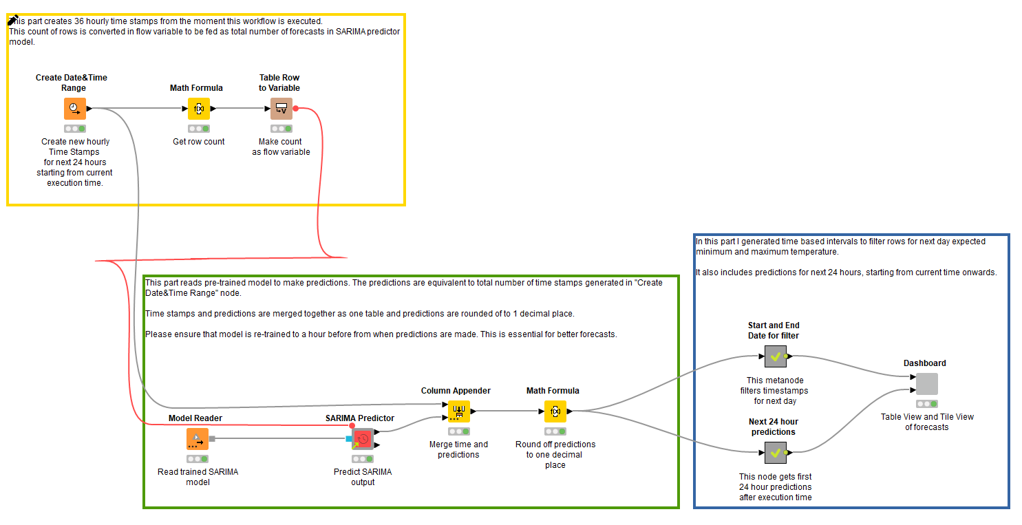
For example, the table populated in Fig. 7 shows hourly forecasts from 15:00 current day till 14:00 next day. And the Tile View shows expected maximum and minimum temperature for the following day.

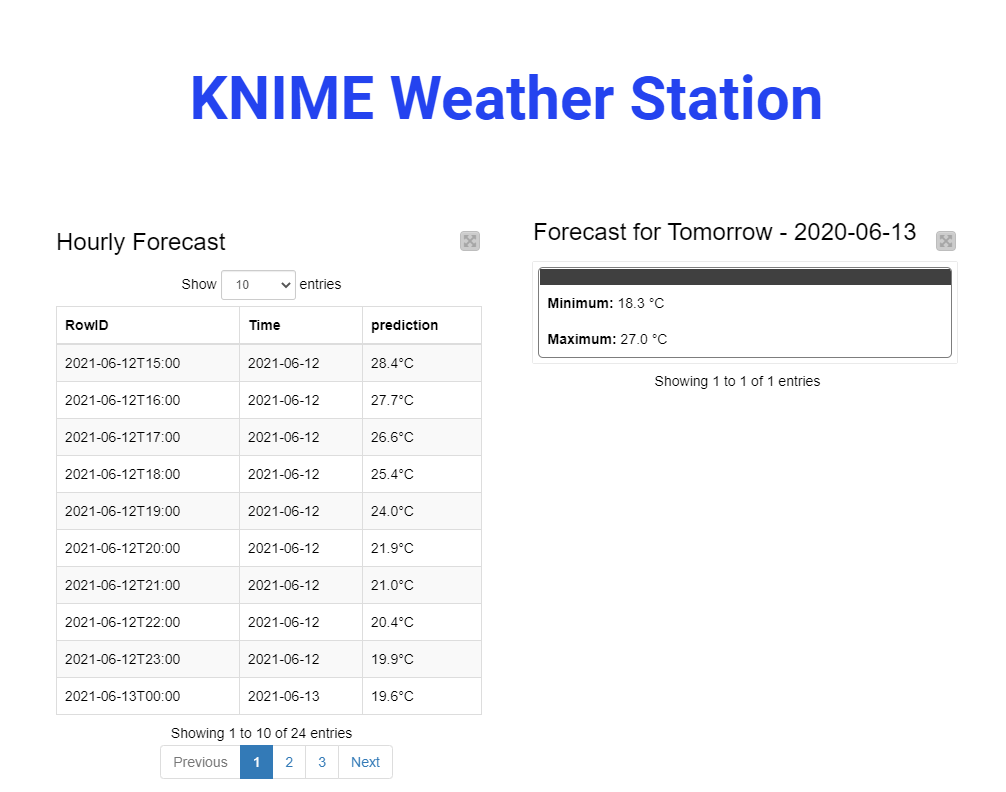
Note. The workflow generating the dashboard in Fig.7 can be found on the KNIME Hub, KNIME Weather Station Forecasting Dashboard

We have described building a full IoT system, an office weather station, using KNIME Analytics Platform. Our weather station was a complete IoT system in the sense that it went from collecting the weather data via a sensor board to storing and analyzing the same data for next day predictions.

With all the data collected every minute from mid of May to mid of June, and aggregated on an hourly average, we trained a sARIMA model to forecast the average temperature for the next hour given the average temperature values for the past 24 hours. The trained model was then deployed to produce a dashboard for us to consume the maximum and minimum temperatures of the upcoming day along with hourly forecasts for the next 24 hour from current time.

The complicated part was actually to set the Arduino sensor board properly (especially to hang it out of our office window) and to set a reasonable calibration of the sensors on it. After that, building a REST service to import the data into Snowflake, aggregating them, training and deploying the sARIMA model, and building a dashboard was easy and - thanks to KNIME’s visual programming environment - all codeless.

• Read the first part of this project Data Collection from IoT Sensors
• Further reading on time series analysis
  • S.A.R.I.M.A. Seasonal ARIMA Models with KNIME
  • Time Series Analysis with Components