S.A.R.I.M.A. Seasonal ARIMA Models with KNIME

Today we'd like to introduce the theory behind the ARIMA (Auto Regressive Integrated Moving Average) model as well as its seasonally expanded counterpart, the SARIMA model. We will cover how to properly prepare time series data to meet the model’s assumption requirements and demonstrate how to apply this type of model in KNIME Analytics Platform.

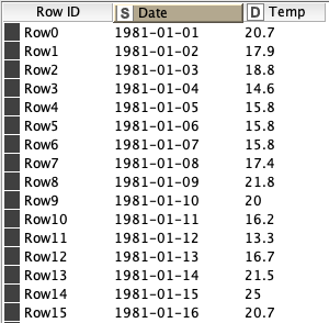
Let’s start by defining Time Series Data, at least in the context of this blog article. Our time series data will be a single variable recorded over and over, typically at even increments of time, although that isn’t always the case as we’ll discuss shortly. This single variable, or single feature in our data is accompanied by a secondary feature, the time stamp. This time stamp simply indicates when the data was recorded. See an example of a Time Series of daily temperature recordings to the right.

Ok, so we have some time series data, so let's toss it all into the ARIMA training algorithm and call it a day! Right? Well not quite. While the ARIMA model is at many times very effective and does not require mountains of data, it does require our time series data to be stationary. Let’s look at what that means.

The first and most important assumption of the ARIMA model is that the underlying data is stationary. In particular weak stationarity is required, although we’ll just call it stationarity as is common practice.

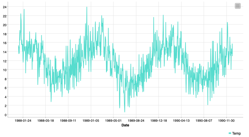
So what is stationarity? It’s simply the idea that regardless of when we look at the data in our time series it has the same “features”. When we talk about weak stationarity these features are mean and variance. In our temperature example data, that would require the mean temperature be the same in both December and July, for example. This obviously isn’t true though, we’ll address how to solve this problem in the next section.

You’ll notice in the title of this article that SARIMA is definitely some kind of acronym, now we’ll dive into the different components of it. Let's start with the AR, we’ll circle back to the S at the end.

Before all of that, let’s introduce some notation. We won’t get too mathy here don't worry!

X_t : We will use X_t to denote the data point in our time series at time t, equivalently X_t-1 will denote the previous data point.

Y_{t :} We will use Y_tto denote the prediction or forecast value of our model at time t, equivalently Y_t-1 will denote the prior forecast.

ɛ_{t :} We will use ɛ_t (pronounced epsilon sub t) to denote the error in our forecast at time t, equivalently ɛ_t-1 will denote the prior error term. This is: ɛ_t=Y_t-X_t

𝝁 : We will use 𝝁 to denote the mean value of our series

The first part of the (S)ARIMA is the auto regressive model. An auto regressive model is one that is based on past (called lagged) values of the target feature. Using our notation from above this means we build a model to predict Xt that looks like:

Y_t=a_{1 ·} X_t-1+a_{2 ·} X_t-2

Where A, B, and C are parameters we fit at train time. Looks a lot like a linear regression, right?!

Unlike the AR and MA parts of the ARIMA model the I does not reference any additional terms to add to our model. Integrated refers to differencing applied to the data before any of the Auto-Regressive or Moving-Average terms are applied.

So what is differencing then? Differencing in this instance means we take the difference between Xtand Xt-1 and we update our series accordingly.

Now instead of having:

X_t, X_t+1, X_t+2 …

We have:

X_t-X_t-1, X_t+1-X_t, X_t+2-X_t+1, …

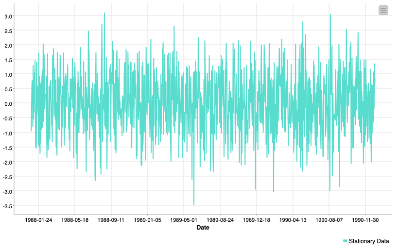
This is the most widely used method for inducing stationarity in time series data. This differencing may happen once or more than once. Differencing once may help remove a linear trend, twice a quadratic trend, and so on. These differencings can be undone automatically at forecast time.

The third part of the (S)ARIMA is the moving average model. Be careful not to mix up this term with the moving average method for smoothing. Like the Auto-Regressive model we add more terms to the regression here. These ones are a bit different though, instead of modeling against lagged values of our target we model against past forecast errors.

Y_t=b_{1 ·} ɛ_t-1+b_{2 ·} ɛ_t-2+𝝁𝜇𝜇

This can be a confusing concept to wrap your head around at first but take my word for it, it’s possible! As an exercise try replacing ɛ_twith ɛ_t=Y_t-X_tand see what happens!

With the baseline ARIMA introduced the upgrade to the Seasonal ARIMA, or SARIMA is a simple expansion.

With the full ARIMA model we apply some differencing to our data, then model with a composite Auto-Regressive Moving-Average model:

Y_t=a_{1 ·} X_t-1+a_{2 ·} X_t-2+b_{1 ·} ɛ_t-1+b_{2 ·} ɛ_t-2+𝝁

After thinking about these equations long enough you’ll notice a limitation. They only increment time steps 1 by 1. The Seasonal ARIMA adds additional terms exactly as the AR and MA parts do, except instead of adding t-1, t-2, t-3, etc., we increment by some seasonal parameter. Commonly this could be 24 hours, 7 days, or whatever fits the pattern you observe in your series.

Doing this you end up with an even longer equation, but still at heart, a regression:

Y_t=a_{1 ·} X_t-1+a_{2 ·} X_t-2+b_{1 ·} ɛ_t-1+b_{2 ·} ɛ_t-2+A_{1 ·} X_t-24+A_{2 ·} X_t-48+B_{1 ·} ɛ_t-24+B_{2 ·} ɛ_t-48+𝝁

Keep in mind however that the Seasonal ARIMA only incorporates these terms and differencings from one seasonality. This means if your data has both daily and weekly cycles you’ll need to account for them before applying the SARIMA model. Possibly by doing additional differencing of your own!

Like most modeling techniques, the SARIMA has a few hyperparameters that describe the specifics of the model you’re creating, these parameters are often called the orders of the SARIMA model. You’ll typically see them written with the name of the model like this:

ARIMA(p,d,q) ARIMA(2,1,2)

SARIMA(p,d,q)(P,D,Q)S SARIMA(2,1,2)(2,0,2)7

These terms are p, d, and q in the standard ARIMA and additionally P, D, and Q in the SARIMA.

p (Auto-Regressive Order): denotes the number of lagged value terms we used in the standard auto-regressive component of our model.

d (Order of Differencing): denotes the number of times we applied standard differencing to our before modeling.

q (Moving-Average Order): denotes the number of past error terms we used in the standard moving-average component of our model.

P, D, and Q are then the seasonal counterparts. Simply the number of seasonal terms or seasonal differencings we apply to our data. They’re commonly called the Seasonal Orders. An intuitive expansion!

*Note that the Seasonal Differencing D can be used to address seasonal patterns in our data and induce the stationarity our model requires. Similar to how standard differencing d could address trends in the data.*

S (Seasonal Period): This is the length of the seasonal cycle based on the number of data points. For example hourly data would make a daily seasonality 24. Daily data would make a weekly seasonality 7. Be careful not to use very long seasonalities as they require more data and train time.

The SARIMA, and equivalently the ARIMA, model can be easily applied in KNIME Analytics Platform. What you see in the screenshot is what we call a Component. In just about every way it is usable like a node, except inside it is composed of a KNIME workflow that you can tweak and edit as needed!

The SARIMA Learner component performs a few checks of your data, and through the KNIME Python Integration trains a (S)ARIMA model with the given orders. It couldn’t be easier to get into SARIMA modeling.

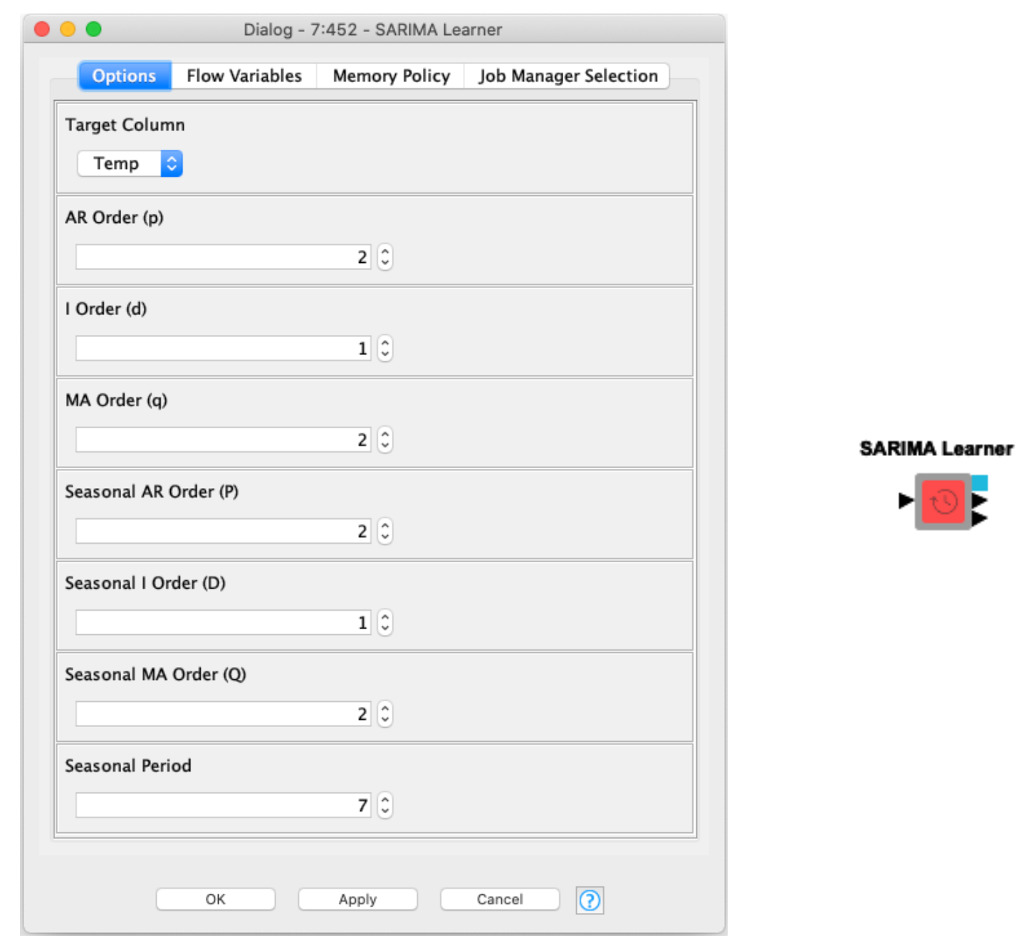
Now, thanks to the Conda Environment Propagation node using this component is easier than ever, under the hood the StatsModels package is used to fit the SARIMA model in Python. This addition allows the component to install the required package directly for you if it is needed, no Python interaction is required!

The SARIMA Learner component has three outputs, from top to bottom:

1. The model port: Connect this to the SARIMA Predictor to generate the future forecasts.
2. Model statistics: Information on the fit coefficients, R2, and other metrics from train time.
3. Residuals: Residuals or forecast errors when applied to our train set, when analyzing these we’d hope to see them looking like white noise, suggesting there is no more information to extract from our data.

Generating forecasts with the SARIMA model is even simpler than training our model. Simply attach the model port from the learner to the predictor and select the number of forecasts to generate! If your data was hourly 24 periods will be one day. If your data was daily 7 periods will be one week.

The SARIMA Predictor component has two outputs, from top to bottom:

1. A table of forecasted values and their standard errors.
2. A table of in sample predictions, this output is only activated if a standard ARIMA model is trained. That being one with no seasonal parameters.

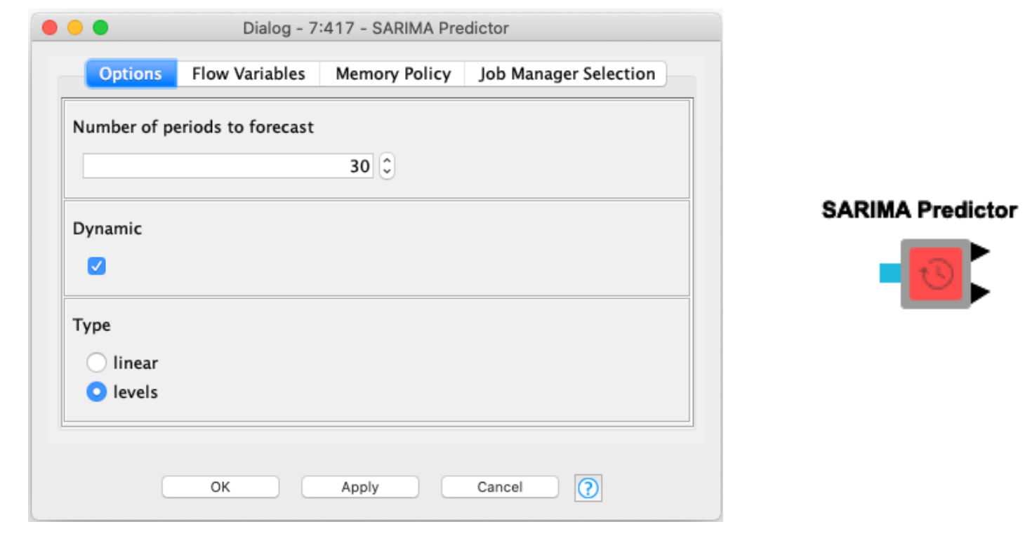
There are two additional options in the configuration. To explain briefly:

• Dynamic: This only affects the in sample prediction, that second table output. If enabled in-sample forecasts will use prior forecast values to generate values. If unchecked true values will be used.
• Type: This only affects (S)ARIMA models that employ differencing. If linear is selected the output forecast values will still be from the differenced series. If levels is selected those values will be transformed back into their original undifferenced state.

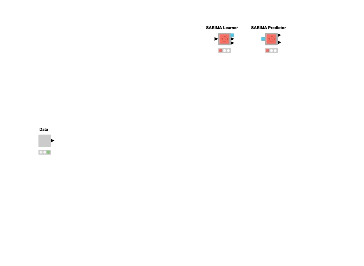
The gif below shows how to assemble the SARIMA Learner and Predictor components into a workflow.

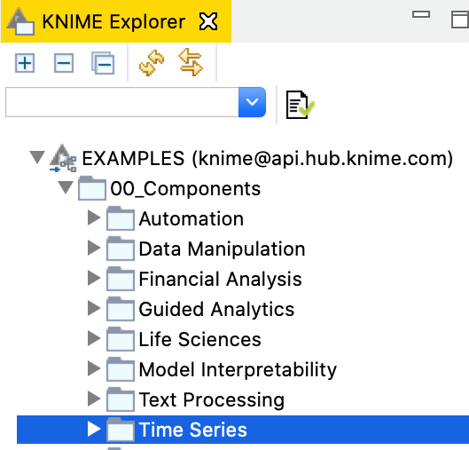
These components can be found both on the KNIME Hub and directly through the KNIME Analytics Platform through the Example Server.

If you like to learn more about Time Series Analysis and the ARIMA models I recommend checking out this early blog post about Building a Time Series Application!

• Time Series Components on Hub
• Blog article, Building a Time Series Analysis Application
• Time Series Workshop on KNIMETV