Multivariate Time Series Analysis: LSTMs & Codeless

Forecasting models are used in many different fields and applications. For example, to predict the demand of a product based on its demand in the last days, weeks, or years. In real life, however, additional time varying features should be included in the model, for example the demand of a related products, as their impact on the predicted value can change over time as well.

Time series analysis applications like these, including past history of more than one feature, belong to the class of multivariate time series problems and recurrent neural networks (RNN) are a great way to solve multivariate time series problems.

In this blog post we’d like to show how Long Short Term Memories (LSTM) based RNNs can be used for multivariate time series forecasting by way of a bike sharing case study where we predict the demand for bikes based on multiple input features.

Univariate time series: Only the history of one variable is collected as input for the analysis. For example, only the temperature data collected over time from a sensor measuring the temperature of a room every second.

Multivariate time series: The history of multiple variables is collected as input for the analysis. For example, in a tri-axial accelerometer, three accelerations are measured over time, one for each axis (x,y,z).

In our example, we use the London Bike Sharing dataset from Kaggle. The dataset has 10 columns including timestamp, count of new bike shares (cnt), as well as additional independent features like the real temperature in °C (t1), the felt temperature in °C (t2), or whether it is a holiday day or not (isholiday). Below an overview of the different input features

• "timestamp" - timestamp field for grouping the data
• TF= "cnt" - the count of a new bike shares
• F₁="t1" - real temperature in C
• F₂="t2" - temperature in C "feels like"
• F₃="hum" - humidity in percentage
• F₄="windspeed" - wind speed in km/h
• F₅="weathercode" - category of the weather
• F₆="isholiday" - boolean field - 1 holiday / 0 non holiday
• F₇="isweekend" - boolean field - 1 if the day is weekend
• F8="season" - category field meteorological seasons: 0-spring ; 1-summer; 2-fall; 3-winter

The count of bike shares (TF) can be interpreted as the demand for bikes at a given time t, as defined by the timestamp feature. The time granularity is hours, that is each record in the dataset refers to the demand for bikes at each hour in the time window used for the data collection. The goal here is to predict the demand for bikes based on past demand values, as well as other features’ past values.

This case study, can therefore be framed as a supervised learning problem. The past demand, i.e. the count of the new bike shares, and the past values of the other features over the last 10 hours represent the input. Our target is to predict the demand for bikes in the next hour.

We decided to go for a many-to-one recurrent neural architecture. This is a commonly used neural architecture, processing sequences of n vectors of input features and producing the output only after the whole sequence of feature vectors has passed through. Furthermore, there are three types of architectures to choose from, when processing sequential data through a recurrent network during training:

• Many-to-many architectures: In this case the input and the target are sequences of vectors. There are two ways how this can be implemented. Either each vector of the sequence produces a response at each time t. Or the input sequence is first processed step by step by a recurrent layer, extracting a dense representation of the input sequence, before another recurrent layer starts generating the output sequence.
• Many-to-one architectures: Only the processing of the last feature vector triggers the network response.This is the type of architecture we have adopted to implement the solution for this case study. Here the input is a sequence of feature vectors, but the output is just one value or vector.
• One-to-many architectures: In this case the input is just a fixed tensor and the output is a sequence of vectors. An example for this kind of architectures is image captioning.

Tip: During deployment a many-to-one architecture can be used to generate a sequence by creating an input sequence including either one or multiple predicted values.

To get started with recurrent neural networks and LSTMs we recommend the following blog posts:

• Understanding LSTMs
• Text Generation with LSTMs

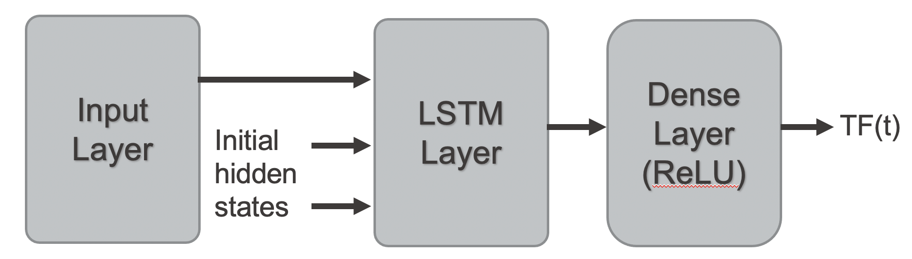
We chose to use a many-to-one LSTM based RNN. This network consists of an input layer to accept the data sequence, an LSTM layer (implementing the many-to-one layer) to process the sequence, and a dense layer with activation function ReLU to predict the next value of the target feature. Figure 1 shows the architecture.

In figure 2 you can see the focus on the many-to-one behavior of the LSTM layer. The graphic shows you the LSTM layer of the network in a so-called unrolled way, where the last 5 time steps are taken into account.

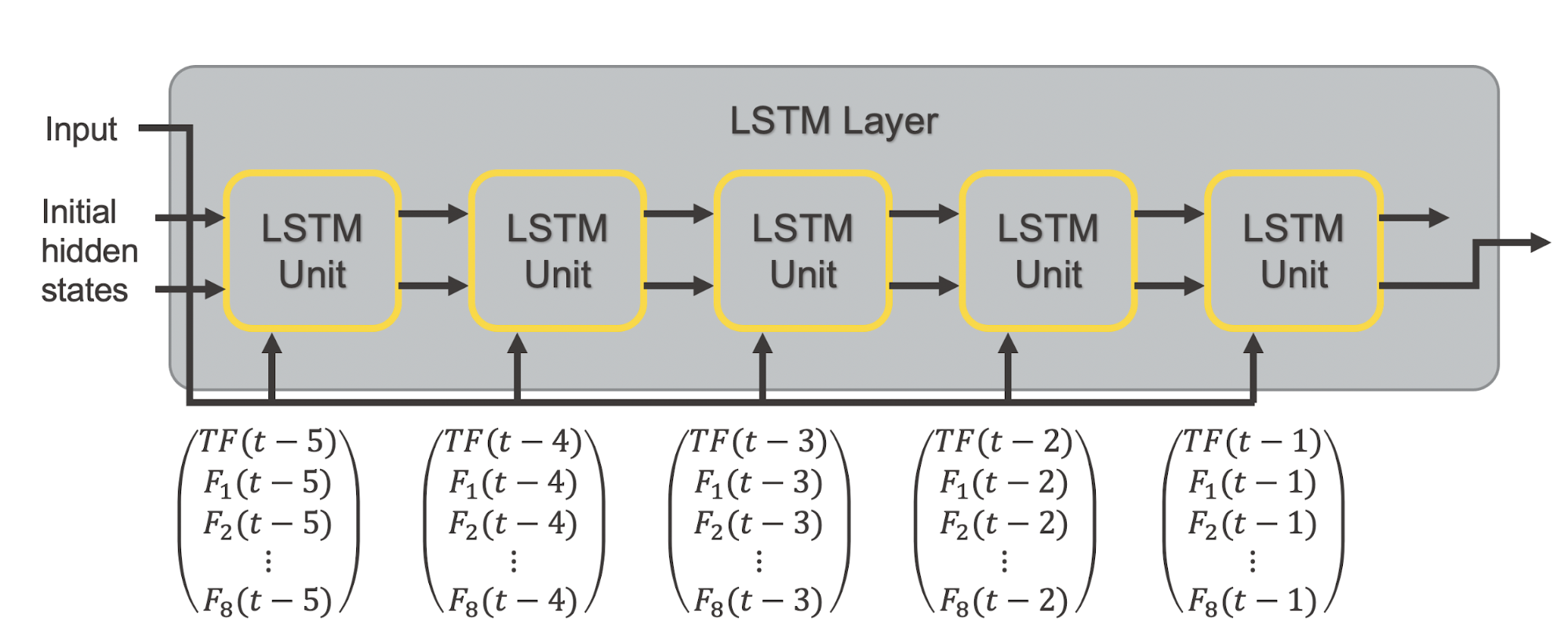
The layer starts, taking into account the feature vector at time t-5 and some initial hidden states. Remember that the feature vector at time t-5 includes the demand value as well as the values for all other features at time t-5. Based on this input, the hidden states of the LSTM unit are updated and fed into the next copy of the LSTM unit together with the feature vector at time t-4 and so on until time t-1.

After processing all feature vectors from the previous 5 time steps, the hidden states should be able to feed the necessary information into the output dense layer with activation ReLU to predict the demand value for the next time step t.

A network like this needs a training set with sequences of 5 feature vectors associated with the demand at the following time step.

There are many ways in which the data can be used. For example, information such as season, isweekend or isholiday is already known for the next day and could be used as additional input feature to add richness to the analysis.

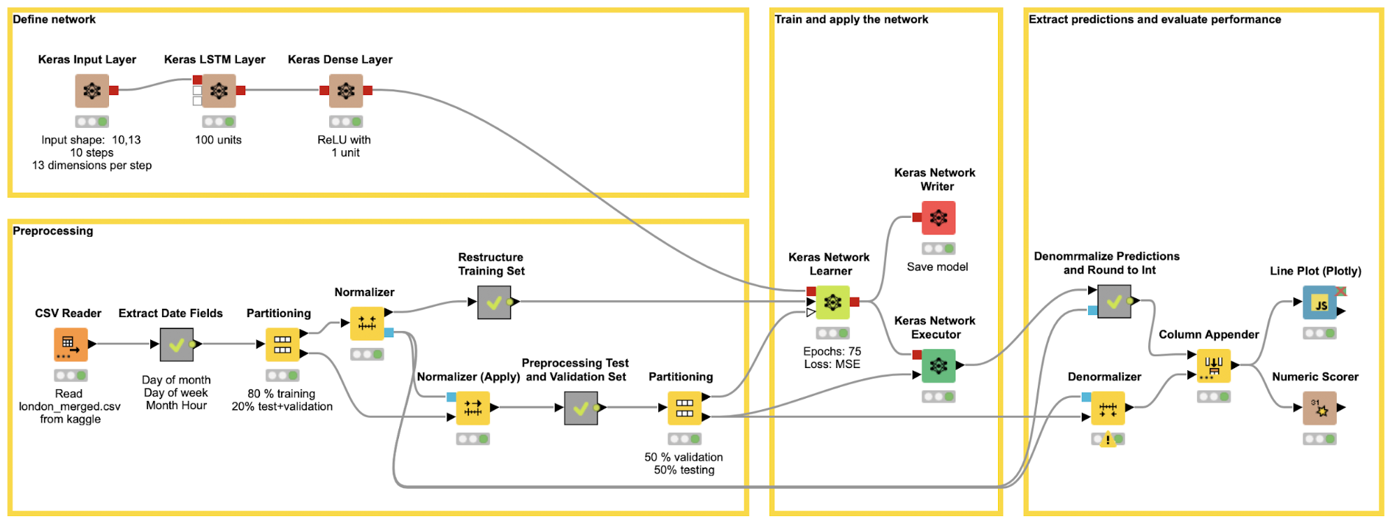
The workflow in figure 3 covers all steps, from reading, preprocessing, defining and training the network, through to executing the network on the test set and evaluating its performance.

Let’s look at the different steps in detail.

The workflow starts by reading the london_merged.csv file using the new (faster) CSV Reader node. (Read more about the new File Handling framework in this blog article.) Next, some time features are extracted from the timestamp field (day of month, day of week, month and hour) using the Extract Date&Time Fields node.

After removing the timestamp column, we are left with 13 attributes. The data are then split in two subsets - one for the training and one for the test and validation sets. Next the data is normalized using the Normalizer node for the training set and Normalizer (Apply) node for the other subsets.

In our case study we adopted sequences of length n=10. This means each training sample should include an input matrix consisting of the feature vectors of the last 10 time steps and the associated target value.

Let’s make a small example for this. Let’s say we have a multivariate time series, with values from three sources x, y, z, and let’s say we make the prediction based on the previous 5 time steps. In this case the input matrix could be organized as follows.

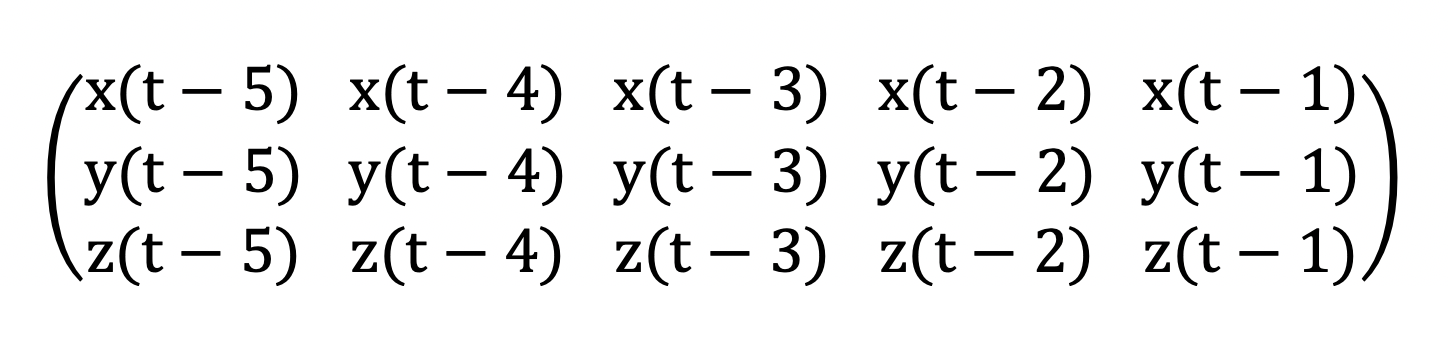
This matrix has shape “5,3”, 5 along the time dimension and 3 along the feature dimension.

In KNIME Analytics Platform this matrix can be created by the Keras Network Learner node based on a vector obtained by concatenating the cells in the matrix above in the following order:

x(t-5), x(t-4), x(t-3), x(t-2), x(t-1), y(t-5), y(t-4), y(t-3), y(t-2) , y(t-1), z(t-5) z(t-4), z(t-3), z(t-2), z(t-1)

That is one feature after the other, with values sorted from the latest to the most recent. We then group all these values within a collection cell and feed them into the network. The layer accepting the input data is usually the Keras Input Layer node. If the Input shape is set as “5,3” in the configuration window of the Keras Input Layer node, then the Keras Network Learner node will convert the values in the collection cell automatically into the desired matrix.

The creation and resorting of such vectors is performed in the “Restructure Training Set” and “Restructure Test and Validation Set” metanodes. Figure 4 shows you the content of the “Restructure Training Set” metanode, which is similar to the content of the “Restructure Test and Validation Set” metanode.

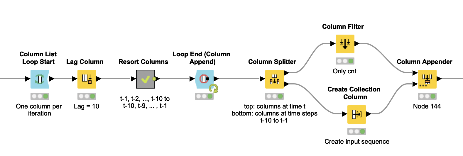
The metanode starts with a loop on the dataset columns. At each iteration one column is processed. The Lag Column node in the loop body - between the Loop Start node and the Loop End node - creates the sequence of n=10 past values of the current column by setting a lag value of 10. The times series produced by the Lag Column node follows this order:

x(t-1) x(t-2) x(t-3)... x(t-9) x(t-10)

The network, however, needs an input sequence in time increasing order, such as:

x(t-10) x(t-9) … x(t-3) x(t-2) x(t-1)

The “Resort Columns” metanode resorts the sequence appropriately. The output of the Loop End (Column Append) node has the sorted sequences of feature vectors and the corresponding targets, as demand values at the next time step.

The table is now split over time: on one side all columns with current values at time t; on the other side all columns with past values at t-10, t-9, …, t-1.

We now look at the table that contains all the columns with current values, and remove all columns with the exception of column “cnt”, which contains the bike demand at day t, what is our target value. We have created the input sequences on one side and the corresponding target on the other. The sequences of the previous feature vectors are aggregated into collection cells, using the Create Collection Column node. Finally, the two parts are rejoined together with the Column Appender node. Our training set is now ready to go.

For this case study, we opted for a basic RNN structure that can be optimized and improved by stacking multiple LSTM layers, including regularization techniques like dropout to avoid overfitting, etc.

The simple network we implement here consists of three layers:

1. An input layer to define the input shape implemented via a Keras Input Layer node. In the case of time series, the input shape is a tuple, represented as n, m, where n is the length of the sequence and m, after the comma, is the size of the feature vector at each time step. In our example, the input shape is 10,13.
2. An LSTM layer implemented via a Keras LSTM Layer node. In a many-to-one architecture we only need the output after the sequence of input vectors has been processed. Therefore the checkbox “Return sequences” is not activated. For the setting option “Units” we used 100.
   Note: LSTMs memorize previous information in the state cell C(t) and produce an output vector h(t). C(t) and h(t) have the same size. The "Units" parameter here refers to the size of such a vector. Therefore the setting “Units” does not refer to the sequence length and shouldn’t be confused with the number of LSTM units in Figure 2, where we use LSTM Unit to describe one copy of the LSTM layer in the unrolled representation.
3. An output layer implemented via a Keras Dense Layer node using the activation function ReLU.

In Figure 3 you can see how this network is built using the sequence of brown nodes in the top left corner of the workflow. Each brown node builds a layer of the network.

Tip: The activation function ReLU is 0 for all negative values and the identity function for all positive values. In our book Codeless Deep Learning with KNIME we describe commonly used activation functions and give some tips on when it is convenient to use which.

Now that we have preprocessed the data and defined the network, we can train the network using the Keras Network Learner node. The configuration window of the node makes it easy to set all training parameters. Here are the settings for this case study:

Now that we have a trained model we can build a second workflow for the deployment.

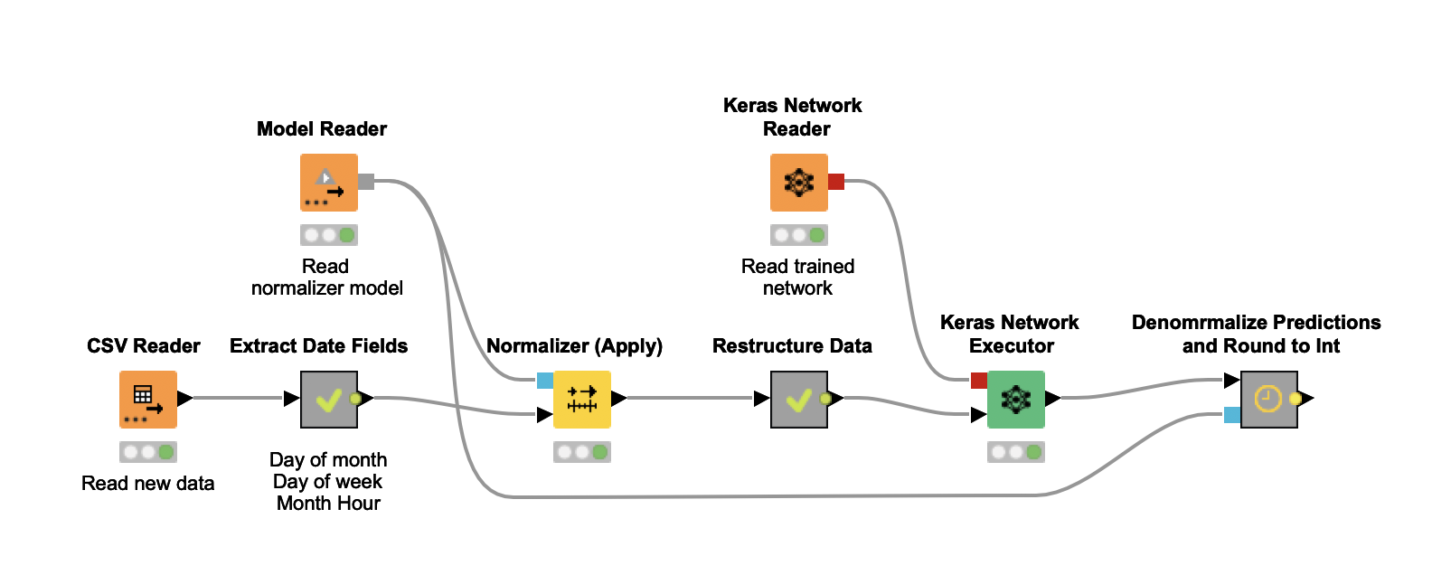
Figure 6 shows you a simple deployment workflow that predicts the demand for the next hour based on the demand and the other features in the last 10 hours.

The workflow reads the new data and performs the same preprocessing steps as in the training workflow. This means extracting fields from the timestamp, using the same normalization, creating the feature vectors and aggregating them into one vector, so that the Keras Network Executor node can create the input matrix. Then the trained network is applied and the predicted value gets denormalized and rounded.

• The training workflow and the deployment workflow we have used in this blog article are both freely available for you to download from the KNIME Hub.
• Check out our Codeless Deep Learning with KNIME book to learn more about the many different options to build, train, and deploy a deep learning network using KNIME Software.

We started with a quick introduction to multivariate time series i.e. times series with multiple variables at each time step. Step by step, you learned how to train a demand prediction model for a multivariate time series using a many-to-one, LSTM based recurrent neural network architecture.

You are now familiar with all the necessary steps to solve your own multivariate time series problem with RNNs. This means all the steps starting from preparing the data - so that the Keras Network Learner node can convert the input into a matrix input - through to training, testing, and deploying your RNN model in KNIME Analytics Platform.

Download more time series analysis workflows or deep learning workflows from our Examples space on the KNIME Hub and try out your new skills!