Lexicon-Based Sentiment Analysis: A Tutorial

How to create sentiment scores for texts based on word sentiment

The main goal of sentiment analysis is to automatically determine whether a text leaves a positive, negative, or neutral impression. It’s often used to analyze customer feedback on brands, products, and services found in online reviews or on social media platforms.

There are different approaches to analyzing the sentiment of texts. In this article we are going to discuss lexicon-based sentiment analysis. We will walk through an example workflow showing you how to build a predictive model that calculates a sentiment score and classifies customer tweets about six US airlines.

Before purchasing a product, people often search for reviews online to help them decide if they want to buy it. These reviews usually contain expressions that carry so-called emotional valence, such as “great” (positive valence) or “terrible” (negative valence), leaving readers with a positive or negative impression.

In lexicon-based sentiment analysis, words in texts are labeled as positive or negative (and sometimes as neutral) with the help of a so-called valence dictionary. Take the phrase “Good people sometimes have bad days.”. A valence dictionary would label the word “Good” as positive; the word “bad” as negative; and possibly the other words as neutral.

Once each word in the text is labeled, we can derive an overall sentiment score by counting the numbers of positive and negative words, and combining these values mathematically. A popular formula to calculate the sentiment score (StSc) is:

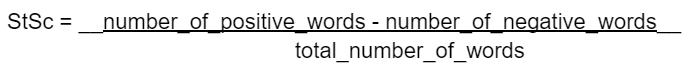
If the sentiment score is negative, the text is classified as negative. It follows that a positive score means a positive text, and a score of zero means the text is classified as neutral.

Note that in the lexicon-based approach we don’t use Machine Learning models: The overall sentiment of the text is determined on-the-fly, depending only on the dictionary that is used for labeling word valence.

Tip: Valence dictionaries are language-dependent and are usually available at the linguistic department of national universities. As an example, consider these valence dictionaries for:

Chinese (http://compling.hss.ntu.edu.sg/omw/)
Thai (http://compling.hss.ntu.edu.sg/omw/) 

The project we now want to walk through involved building a lexicon-based predictor for sentiment analysis. We used a Kaggle dataset containing over 14K customer reviews on six US airlines.

Each review is a tweet annotated as positive, negative, or neutral by contributors. One of our goals is to verify how closely our sentiment scores match the sentiment determined by these contributors. This will give us an idea of how promising and efficient this approach is.

Note. You can download the example workflows for this project from the KNIME Hub. The Machine Learning and Marketing space on the KNIME Hub contains example workflows of common data science problems in Marketing Analytics. The original task was explained in: F. Villarroel Ordenes & R. Silipo, “Machine learning for marketing on the KNIME Hub: The development of a live repository for marketing applications”, Journal of Business Research 137(1):393-410, DOI: 10.1016/j.jbusres.2021.08.036. Please cite this article, if you use any of the workflows in the repository.

Let’s now walk through the different parts of the workflow.

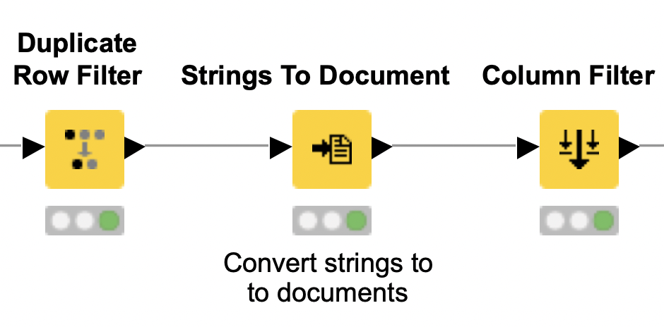
Before building our sentiment predictor, we need to clean up and preprocess our data a little. We start by removing duplicate tweets from the dataset with the Duplicate Row Filter node. To analyze the tweets, we now need to convert their content and the contributor-annotated overall sentiment of the remaining tweets into documents using the Strings To Document node.

Tip: Document is the required type format for most text mining tasks in KNIME, and the best way to inspect Document type data is with the Document Viewer node.

These documents contain all the information we need for our lexicon-based analyzer, so we can now exclude all the other columns from the processed dataset with the Column Filter node.

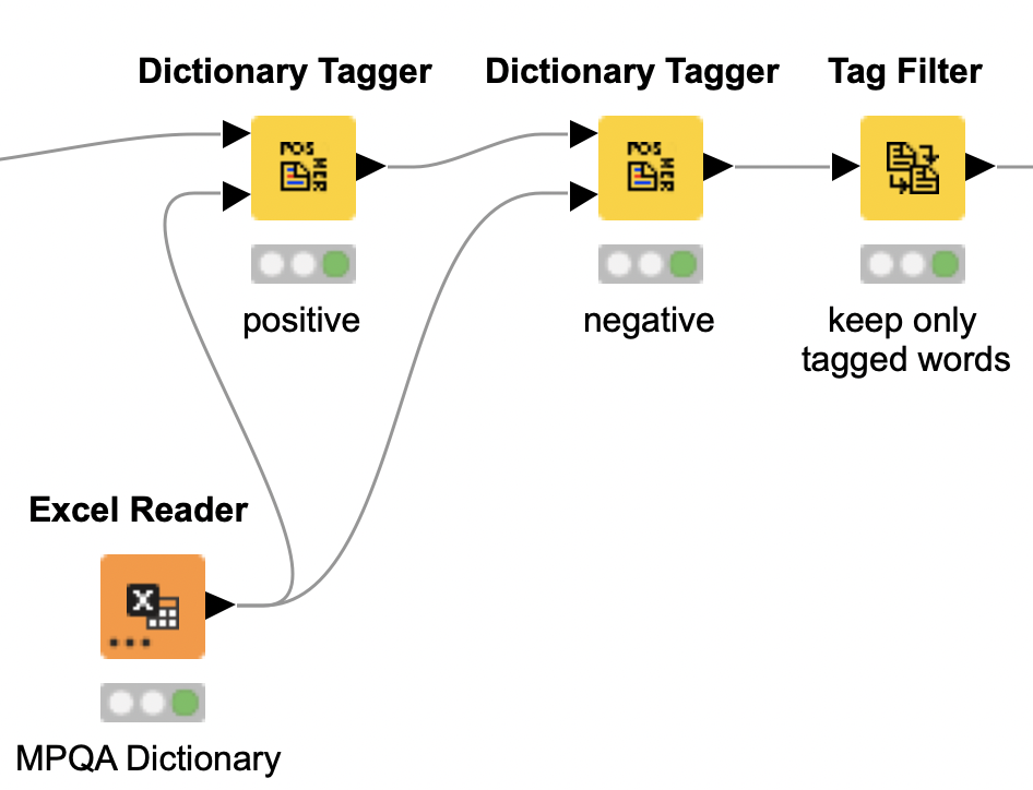
We can now move on and use a valence dictionary to label all the words in the documents we have created for each tweet. We used an English dictionary from the MPQA Opinion Corpus which contains two lists: one list of positive words and one list of negative words.

Tip: Alternative formulas for sentiment scores calculate the frequencies of neutral words, either using a specific neutral list or by tagging any word that is neither positive nor negative as neutral.

Each word in each document is now compared against the two lists and assigned a sentiment tag. We do this by using two instances of the Dictionary Tagger node. The goal here is to ensure that sentiment-laden words are marked as such and then to process the documents again keeping only those words that were tagged (with the Tag Filter node).

Note that since we’re not tagging neutral words here, all words that are not marked as either positive or negative are removed in this step.

Now, the total number of words per tweet, which we need to calculate the sentiment scores (see formula above), is equivalent to the sum of positive and negative words.

What we now want to do is generate sentiment scores for each tweet. Using our filtered lists of tagged words, we can determine how many positive and negative words are present in each tweet.

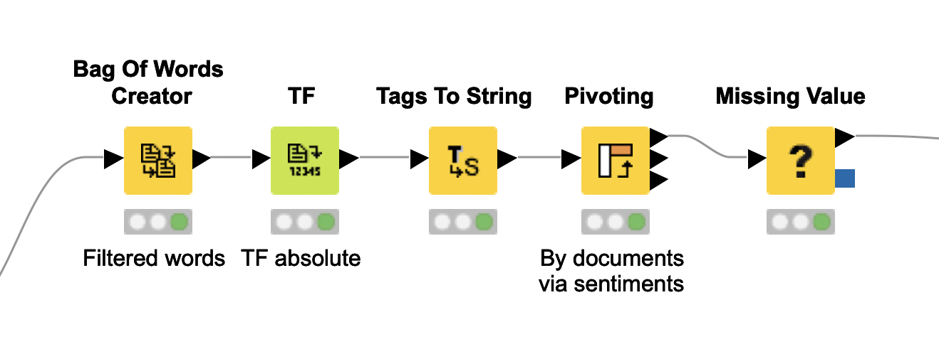
We start this process by creating bags of words for each tweet with the Bag Of Words Creator node. This node creates a long table that contains all the words from our preprocessed documents, placing each one into a single row.

Next, we count the frequency of each tagged word in each tweet with the TF node. This node can be configured to use integers or weighted values, relative to the total number of words in each document. Since tweets are very short, using relative frequencies (weighted values) is not likely to offer any additional normalization advantage for the frequency calculation. For this reason, we use integers to represent the words’ absolute frequencies.

We then extract the sentiment of the words in each tweet (positive or negative) with the Tags to String node, and finally calculate the overall numbers of positive and negative words per document by summing their frequencies with the Pivoting node. For consistency, if a tweet does not have any negative or positive words at all, we set the corresponding number to zero with the Missing Value node. For better readability, this process is encapsulated in a metanode in the workflow.

We’re now ready to start the fun part and calculate the sentiment score (StSc) for each tweet.

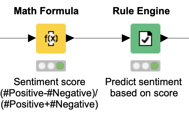
We get our sentiment score by calculating the difference between the numbers of positive and negative words, divided by their sum (see formula for StSc above) with the Math Formula node.

Based on this value, the Rule Engine node decides whether the tweet has positive or negative sentiment.

Since the tweets were annotated by actual contributors as positive, negative, or neutral, we have gold data against which we can compare the lexicon-based predictions.

Remember that StSc > 0 corresponds to a positive sentiment; StSc = 0, to a neutral sentiment; and StSc classification problem.

To perform this comparison, we start by setting the column containing the contributors’ annotations as the target column for classification, using the Category to Class node. Next, we use the Scorer node to compare the values in this column against the lexicon-based predictions.

It turns out that the accuracy of this approach is rather low: the sentiment of only 43% of the tweets was classified correctly. This approach performed especially badly for neutral tweets, probably because both the formula for sentiment scores and the dictionary we used do not handle neutral words directly. Most tweets, however, were annotated as negative or positive, and the lexicon-based predictor performed slightly better for the former category (F1-scores of 53% and 42%, respectively).

After assessing the performance of our predictor, we implemented a second workflow to show how our predictive model could be deployed on unlabeled data. The mechanics of both workflows are very similar, but there are a few key differences.

First, this deployment workflow implements a component named Tweet Extraction, which includes the Twitter API Connector node – to connect to the Twitter API – and the Twitter Search node to query the API for tweets with a given hashtag. We used configuration nodes inside the component to enable users to enter their Twitter credentials and specific search query. Configuration nodes within the component create the configuration dialogue of the components for the Twitter credentials and the search query. By default, the Twitter API returns the tweets from last week, along with data about the tweet, the author, the time of tweeting, the author’s profile image, the number of followers, and the tweet ID.

This process is followed by some post-processing that will help improve visualizations of our data further down the line. On the one hand we want to remove retweets as they can become excessive and impair the legibility of visualizations – and on the other hand – we want to format the tweets’ timestamps to make the visualizations less cluttered.

The process of tagging words in tweets, deriving sentiment scores and finally predicting their sentiments is no different from what we described for the first workflow. However, since we do not have labels for the tweets here, we can only assess the performance of the lexicon-based predictor subjectively, relying on our own judgment.

To help us assess the performance, we implemented a composite visualization that combines (1) the tweets; (2) a word cloud in which the tweets appear with sizes that correspond to their frequency; and (3) a bar chart with the number of tweets per sentiment per date. This visualization is interactive. Users can click different bars in the bar chart to modify the content selection of the word cloud, for example.

In terms of structure, the workflow uses the Document Data Extractor node to retrieve all tweet information stored in the Document column, and the Joiner node to join the profile image back to the tweet. Next, a dashboard produces the word cloud, the bar chart, and a table with all extracted tweets.

Now let’s take a closer look at how this predictor works in practice. Consider at first the content of the following tweet:

@VirginAmerica I

The words “pretty” and “better” were tagged by our predictor as positive; no words were tagged as negative. This led to StSc = 1, meaning the tweet was then classified as having positive sentiment — something with which most annotators may agree. Let’s now take a look at a different example, for which our predictor fails:

@AmericanAir @SKelchlin What kind of  response is this from an airline? "When they can?". How about an apology.

The word “kind” was tagged as positive, even though it does not correspond to a positive adjective in this context, and no words were tagged as negative. Consequently, the tweet was classified as positive even though it in fact corresponds to a complaint.

These examples illustrate a few limitations of the lexicon-based approach: it does not take the context around words into consideration, nor is it powerful enough to handle homonyms, such as “kind”.

Lexicon-based sentiment analysis is an easy approach to implement and can be customized without much effort. The formula for calculating sentiment scores could, for example, be adjusted to include frequencies of neutral words and then verified to see if this has a positive impact on performance. Results are also very easy to interpret, as tracking down the calculation of sentiment scores and classification is straightforward.

Despite its low performance, a lexicon-based sentiment predictor is insightful for preliminary, baseline analysis. It provides analysts with insights at a very low cost and saves them a lot of time otherwise spent analyzing data in spreadsheets manually.

Feel free to download the workflows we have described here and try out the effect of adjusting how sentiment scores are calculated.