Identify Continuous Probability Distributions with KNIME

Before we start conducting statistical tests on our data, we need to know what probability distribution our data follows to improve the efficiency of our machine learning algorithms, enabling proper and faster convergence, and better predictions.

To automatically identify the continuous probability distribution your data follows, we've built an easy-to-use KNIME component. It gives you the five best-fitting distributions that describe your data, as well as probability distributions and probability plots. The component interactive view also displays descriptive statistics for the selected column(s).

All you have to do is use your data as input for this component and select at least one numeric column in the configuration window. The component does the rest of the work for you!

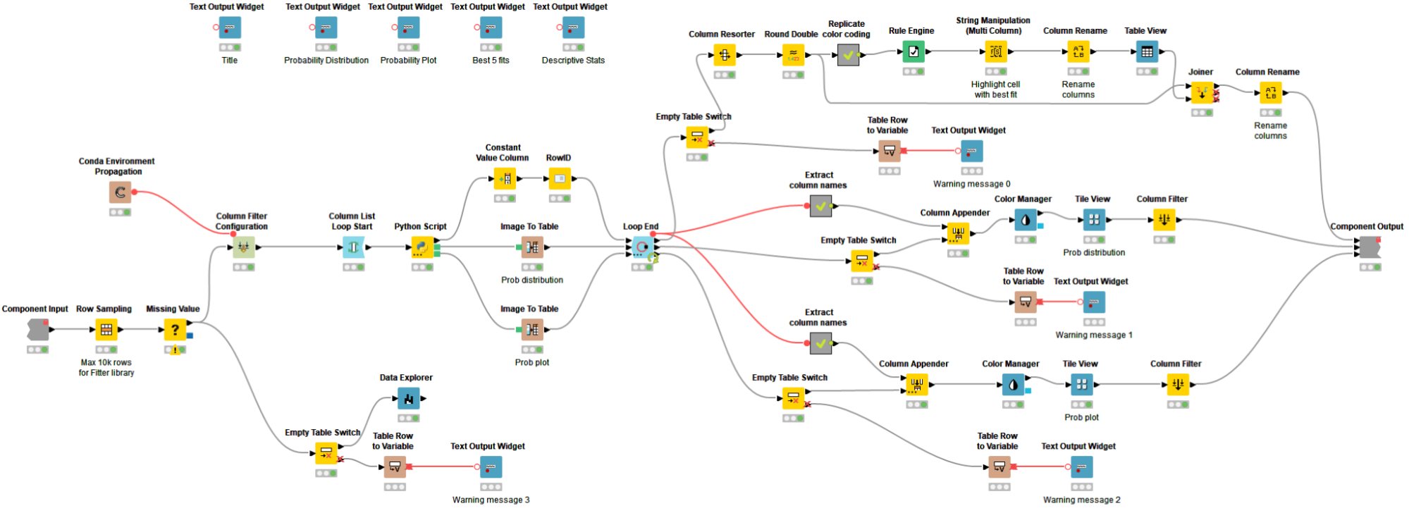
We used the KNIME Python Integration to develop our workflow. To make the workflow easier to share and reuse, we encapsulated it into a component. (Fig. 1).

Tip: Check out How to Set Up the Python Extension and the KNIME Python Integration Installation Guide to know more.

The Continuous Probability Distribution component is a Python-based component and uses the FITTER library in a Python Script node to identify the five best-fitting continuous distributions for the input data. This library imports approximately 80 continuous distributions from Scipy, scans all of them, calls the underlying fit function, and finally returns a statistical score table of the best-fitting probability distributions ranked by the least sum of the squared errors. On the basis of this ranking, the FITTER library generates two visualizations: a probability distribution and a probability plot, which are returned by and displayed in the component interactive view.

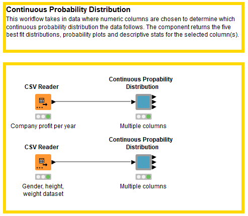
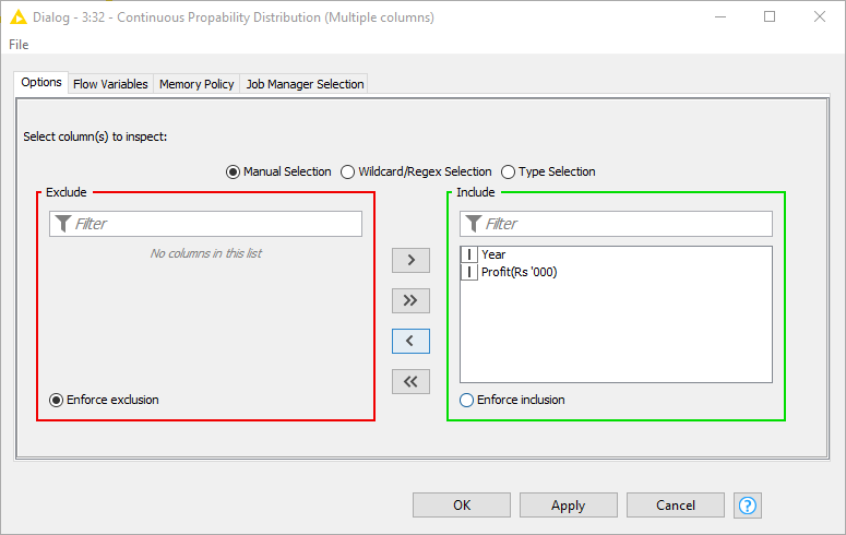
This Continuous Probability Distribution component allows the user to select one or multiple numeric columns in the configuration window (see Fig. 2). In our example workflow, we input a dataset containing information about a company's profit (in thousands of rupees) and the year.

Notice that we also provided a second dataset describing adults by gender, height, weight, and index (Fig. 11). Gender is of type String. The Continuous Probability Distribution component allows only the selection of and distribution fitting for numeric columns, be they of type Integer, Double or Long.

The workflow wrapped inside the component handles missing values, solves the processing limitation (max 10K rows) of the FITTER library by randomly undersampling the input dataset, introduces workflow control logic to handle empty tables, and relies on the Conda Environment Propagation node to install required Python libraries and enhance workflow portability across different OSs (Fig. 13).

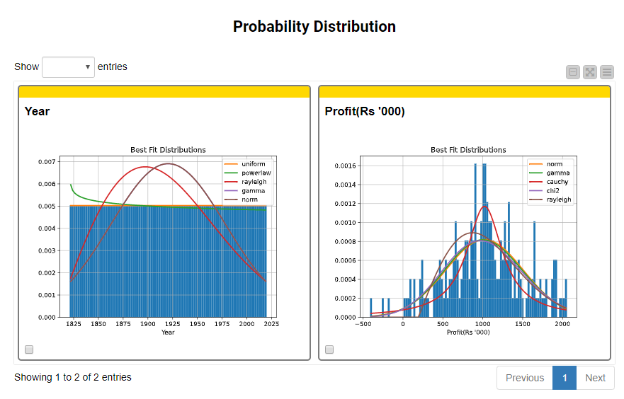
With the help of Widget and View nodes, the component produces an interactive dashboard of the five best-fitting continuous probability distributions that describe the input columns. In our example, the Probability Distribution plots show that Year is best fitted by a uniform distribution, whereas Profit is by a normal distribution (Fig. 14).

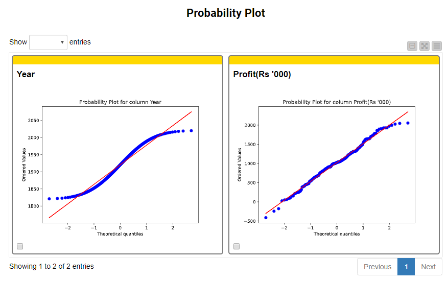
Additionally, the dashboard displays Probability Plots (Fig. 15). Probability plots are used as a graphical technique to assess whether or not a numeric column follows a given distribution. Taking a closer look at the probability plots, we can see that the estimated top probability distributions (i.e., uniform and normal, respectively) are accurate since the observations of both Year and Profit are clustering closely around or on top of the fitting line with the respective shape of the distribution.

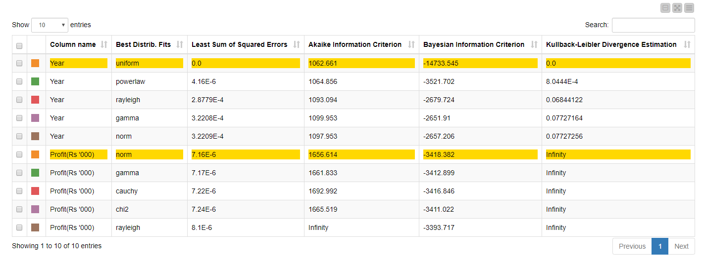
The component also outputs two interesting statistical tables: a score table of the best-fitting probability distributions, and a table containing descriptive statistics.

The first table is sorted by the least sum of the squared errors, i.e., the difference between the predicted (or fitted) and the observed value. The lower the sum of the squared errors, the better the fit of the line (or distribution) to the data. The table also includes scores for the Kullback-Leibler Divergence Estimation, Akaike Information Criterion (AIC) and Bayesian Information Criterion (BIC). The first is a measure of how one probability distribution is different from a second reference probability distribution. If one distribution predicts that an event is possible and the other predicts it is absolutely impossible, then the two distributions are absolutely different and result in a divergence that is infinite. AIC and BIC are two ways to compare statistical models and select the best-fitting one. Lower AIC and BIC scores are an indicator of good model fit (check the links above for a more detailed interpretation of the scores).

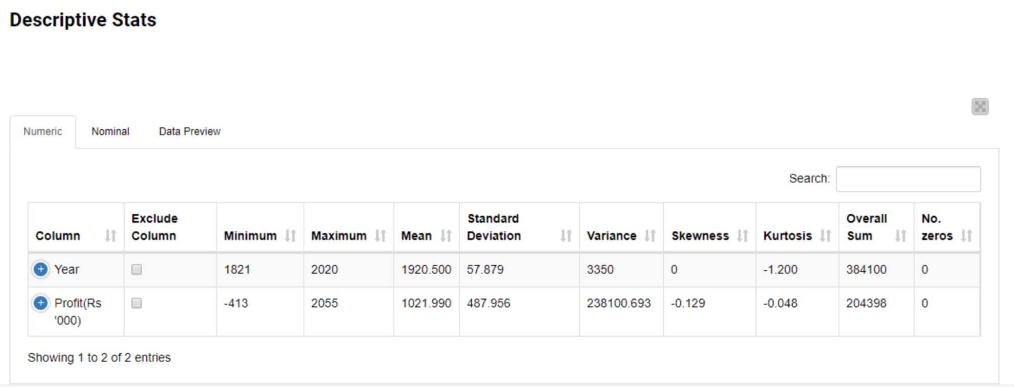
The second table provides a comprehensive and interactive statistical summary (max, min, mean, SD, variance, etc.) of the selected columns.

The knowledge you now gain about your data will help you decide which statistical technique is better-suited and transforming the data distribution to improve the efficiency of ML algorithms becomes much easier! You can download the Continuous Probability Distribution component in this workflow from the KNIME Hub.