What are continuous probability distributions & their 8 common types?

Continuous probability distributions are a framework for modeling and interpreting continuous variables. Examples of continuous variables are: modeling the rate of radioactive decay, or the speed of sound waves, height, weight, blood pressure, cholesterol levels, etc.

In this blog post, we will discuss:

• What is a continuous probability distribution?
• 8 common types of continuous distributions

Probability distributions can be continuous or discrete. 

A discrete probability distribution would have a finite number of distinct outcomes, like the results of rolling a die multiple times or picking a card from a deck repeatedly. For example, when rolling a die multiple times, each roll results in one of six possible outcomes, making it a discrete distribution. You’ll never roll a 1.3 or 5.4.  

A continuous probability distribution could be any one of infinite values in a range. For example, an adult’s height could only ever fall between the values 1 foot and 10 feet but could be any one of the infinite values in between — 5 feet or 5.1 or 5.01 or 5.001. 

Continuous probability distributions are represented by a Probability Density Function (PDF), which describes the shape of the distribution. The PDF describes the likelihood of a random variable taking on specific values within a given range. It essentially outlines how values are distributed across the range, providing a visual depiction of the distribution's shape, such as whether it's symmetric, skewed, or peaked.

Understanding the shape is important because it provides information about the behavior and characteristics of the random variable being studied. 

The probability function is given by the following equation, which describes the probability that x falls between two values (a and b) is equal to the integral (area under the curve) from a to b.In other words, x is a continuous random variable that can take on any value within a given range of values.

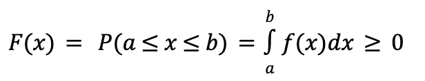
Furthermore, in continuous probability distributions, the probability of x  assuming any specific, exact value is precisely 0. This is due to the infinite number of possible values within a given range, making the probability of landing on one exact value infinitesimally small. 

For instance, consider a continuous probability distribution for women's weight. While the probability distribution across the population suggests that the average woman weighs 60 kg, determining the probability of an individual woman weighing precisely 60 kg is practically impossible.

This is because the chances are exceedingly small, given the continuous nature of the variable; a woman could weigh 60.5 kg, 59.8 kg, or any value within the range. Since measurements on a continuous scale are inherently infinite, pinpointing the probability of a specific measurement occurring becomes impractical.

Often, in the realm of data analysis and statistics, we come across discussions about different types of distributions, such as the normal distribution, exponential distribution, or uniform distribution. These distributions are examples of continuous probability distributions, which describe the likelihood of observing different values within a continuous range of outcomes.

For data scientists, knowing which distribution your data follows influences the choice of appropriate statistical tests and provides insights into the data's characteristics. It also shows us how often the values occur and how to adapt the current data distribution to align with recognized distribution patterns. This helps to significantly improve the efficiency of ML algorithms ‒ proper and faster convergence and better predictions.

In this section, we’ll review the theoretical definition and graphical visualization of 8 common continuous probability distributions, examine examples, and discuss why each distribution is important.

Normal distribution, also known as Gaussian distribution, is often used to approximate the distribution of many real-world phenomena such as height, weight, test scores, etc. In a normal probability distribution, most of the observations cluster around the central peak. In contrast, values further away from the mean taper away symmetrically on both sides and are less likely to occur.

The area under the normal distribution curve represents probability and sums to one. The normal distribution is symmetric and often called the “bell curve” because the graph of its probability density looks like a bell. The only two parameters to describe a normal distribution are the mean and standard deviation. 

When these parameters change, the shape of the distribution also changes (see below). For a perfectly normal distribution the mean, median, and mode will be the same value, visually represented by the peak of the curve.

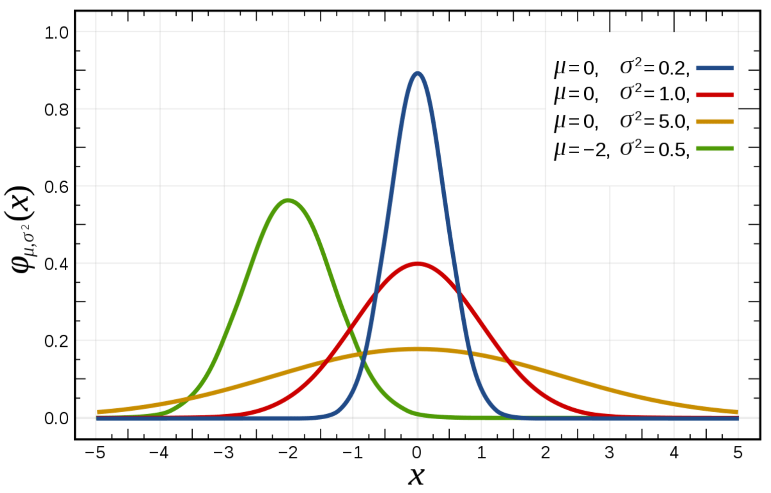
One of the key characteristics of a normal distribution is that it is unimodal i.e., it has only one high point (peak) or maximum, and its tails are asymptotic which means that they approach but never quite insect with the x-axis. This is important because, in theory, even very extreme values can occur by chance.

The formula of the PDF to calculate a normal distribution is given below:

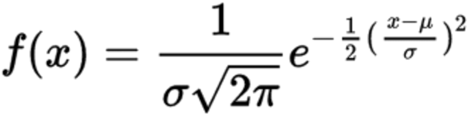
Where f(x) is the probability density function, x is the value or variable of the data that is examined, μ is the mean, and σ is the standard deviation.

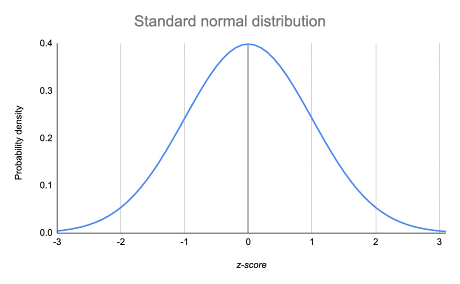
When standardizing a normal distribution, the mean is fixed to 0 and the standard deviation is fixed to 1. The standard normal distribution, also called z-distribution, is a special form of normal distribution. Any normal distribution can be converted to a standard normal distribution using the formula:

z = (x - μ) / σ

You may be wondering why normal distributions are so popular. 

The popularity of normal distributions arises from their mathematical properties, versatility in modeling diverse phenomena, and widespread application in statistical theory and practice. It's a consensus among statisticians, scientists, and practitioners in various fields that normal distributions offer a valuable framework for understanding and analyzing data.

Some of the credit goes to the Central Limit theorem. The central limit theorem states that the distribution of sample means approximates a normal distribution as the sample size gets larger, regardless of the population's distribution. 

Moreover, contributing to the popularity of normal distributions is the simplicity of working with them since it requires only two parameters to describe the distribution. Almost all of the inferential statistics, such as t-tests, ANOVA, simple regression, and multiple regression rely on the assumption of normality.

Even though normal distributions can often be the star of the show, blindly assuming normality without verifying the actual distribution of your data can lead to inaccurate predictions and flawed conclusions, particularly in predictive modeling. Real-world datasets often deviate from normality, and failing to account for this can result in biased estimates and poor model performance. So, it's always advisable to test and find out what distribution your data follows instead of just blindly going with the popular guy!

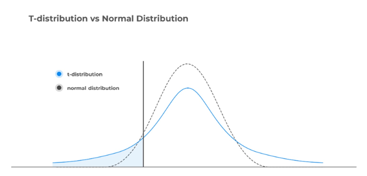
t-distribution, also known as student’s t-distribution, is a kind of distribution that looks almost identical to the normal distribution curve. Indeed, the graph is symmetric and resembles a bell-shaped curve but thicker in the tails indicating that this distribution is more prone to producing values that fall far from its mean. 

The choice between the t-distribution and the normal distribution depends on the characteristics of the data at hand. The t-distribution is favored over the normal distribution in scenarios where the sample size is small, typically less than 30, and the population standard deviation is unknown. 

In such cases, the t-distribution accommodates the additional uncertainty inherent in small sample sizes and the need to estimate the population standard deviation from the sample. This preference arises because the t-distribution's shape is more spread out in the tails compared to the normal distribution, reflecting the greater variability expected in smaller samples.

Let's consider a small example to better understand when the t-distribution can be used. 

Let’s say we want to explore the distribution of cars sold by a dealer in a month or a day, the first step would be to gather the actual data, such as recording the number of cars sold each day or each month. Then, you can create a histogram or another type of plot to visually represent the distribution of these data points. This graphical representation will give you insights into how the data are spread out and whether they follow a particular pattern or distribution.

After examining the distribution graphically, you might then choose to fit a probability distribution to the data. The choice of distribution would depend on various factors, including the shape of the data distribution, the sample size, and any assumptions about the underlying population.

For instance, if the data distribution closely resembles a bell curve (the shape of the normal distribution), and the sample size is large enough, you might decide to use the normal distribution to model the data. However, if the sample size is small or if the data distribution deviates significantly from a bell curve, you might need to consider alternative distributions, such as the t-distribution.

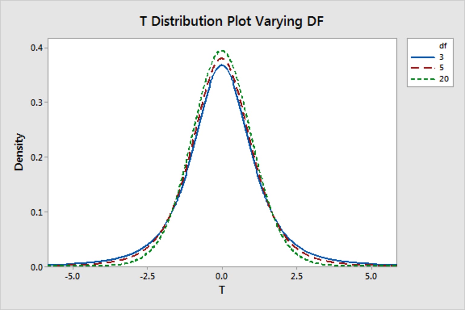
The t-distribution has only one parameter – the degree of freedom (df). With n as the sample size, the degrees of freedom refer to the number of independent observations and can be computed by the formula:

v=n-1

With a sample of 8 observations and using the t-distribution, we would have 7 degrees of freedom. In the graphic below, we see that as the degrees of freedom increase, the t-distribution resembles the normal distribution, with the tails becoming thinner and the peaks taller.

The formula of the PDF to compute the t-distribution is:

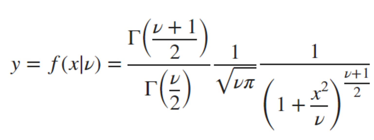
Where the degrees of freedom and Γ( · ) is the Gamma function. The result y is the probability of observing a particular value of x from the t-distribution with degrees of freedom.

Notice that in the absence of explicit normality of a given distribution, a t-distribution may still be appropriate if the sample size is large enough for the central limit theorem to be applied. Indeed, for large sample sizes (>30 observations), the t-distribution looks like the normal distribution and is considered approximately normal.

The t-distribution is often used to find the critical values for a confidence interval when the data is approximately normally distributed. It is also useful in finding the corresponding p-value from a statistical test such as t-tests or regression analysis.

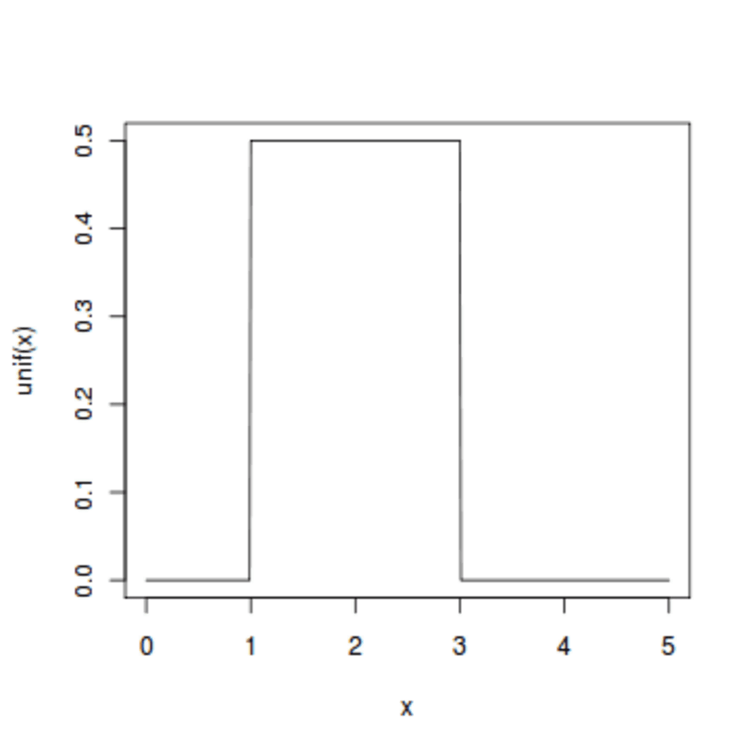
Uniform distribution is also known as rectangular distribution because of its shape (Fig. 5). It refers to an infinite number of equally likely measurable values where the continuous random variable can take any value that lies between certain bounds. 

The bounds are defined by two parameters, a, and b, which are the minimum and maximum values. The interval can either be closed (e.g. [a, b]) or open (e.g. (a, b)). Therefore, the distribution is often abbreviated U(a, b), where U stands for uniform distribution. It is a symmetric probability distribution where all outcomes have an equal likelihood of occurring.

To understand this distribution, let’s see an example. Imagine you live in a building that has an elevator that takes you to your floor. From experience, you know that once you push the button to call the elevator, it takes between 10 to 30 seconds (the lower and upper bounds, respectively) for you to arrive at your floor. This means the elevator arrival is uniformly distributed between 10 to 30 seconds once you hit the button.

The PDF to compute uniform distribution is:

Where f(x) is the probability density function and is constant over the possible values of x, a is the lower bound, and b is the upper bound.

Exponential distribution is used to model the time elapsed before a given event occurs. It describes the time between events in a Poisson process, i.e., the process in which events occur continuously and independently at a constant average rate. For instance, the exponential distribution can represent the time between consecutive arrivals of buses at a bus stop, where arrivals are independent and occur at a constant average rate.

This distribution is frequently used to provide probabilistic answers to questions concerning, for example, the time associated with receiving a defective part on an assembly line, the time elapsed before an earthquake occurs in a given region or the waiting time before a new customer enters a shop.

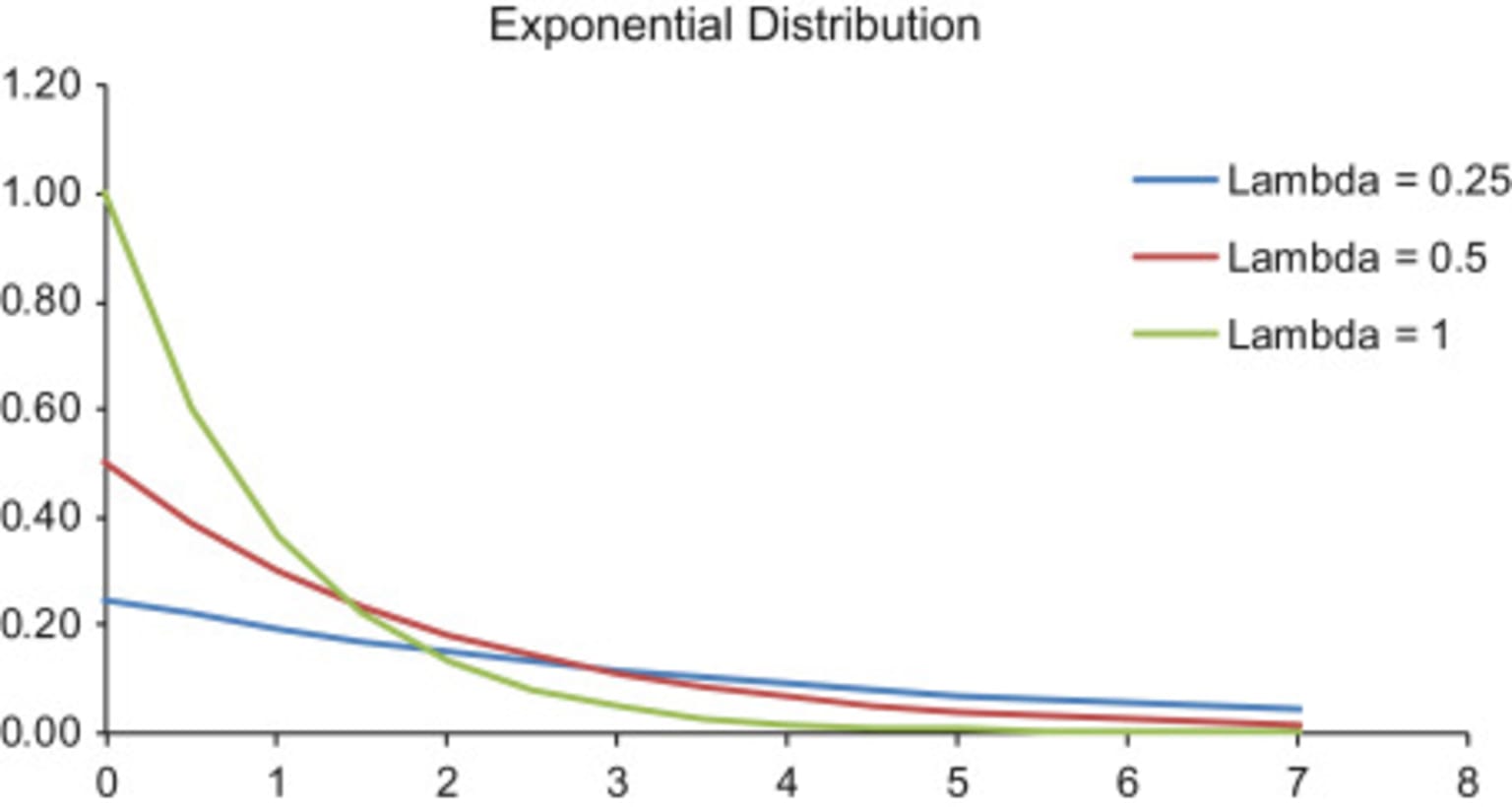
The key parameter of the exponential distribution is λ, known as the rate parameter. The rate parameter indicates how quickly the decay of the exponential function occurs. Changing the decay parameter affects how fast the probability distribution converges to zero. As λ increases, the distribution decays fast; i.e., we obtain a steeper curve. 

We can see this in the case where λ is equivalent to 1 (Fig. 6). Decreasing the λ value translates into slower decay, and when λ is close to 0 (0.1 or 0.2), the decay is minimal. Figure 6 shows the graph of an exponential distribution for different values of lambda:

The PDF to calculate exponential distribution is:

Where f(x; λ) is the probability density function, x is the random variable, and λ is the rate of the distribution.

One important property of the exponential distribution is the memoryless property. This property helps understand the average behavior of exponentially distributed events occurring one after the other. According to this property, the past has no significance on the distribution’s future behavior. That is, irrespective of how much time has already elapsed, every instance is a new beginning. 

Due to the memoryless property, while observing several events in succession with exponentially distributed interarrival times, the expected time until the next event is always 1/λ, no matter how long we have been waiting for a new arrival to occur.

It’s noteworthy to keep in mind that the exponential distribution is related to the Poisson distribution. Suppose that an event can occur more than once and the time elapsed between two successive occurrences is exponentially distributed and independent of previous occurrences (memoryless property), then the number of occurrences of the event within a given unit of time has a Poisson distribution.

The Chi-square distribution is widely used in inferential statistics for the construction of confidence intervals and hypothesis testing. The shape of a chi-square distribution is determined by the parameter k, which represents the degrees of freedom. 

Similar to the t-distribution, the chi-square distribution is closely related to the standard normal distribution. This is because if we sample from n independent standard normal distributions and then square and sum the values, we will obtain a chi-square distribution with k degrees of freedom, where k equals the number of independent normal distributions sampled (n). The values in the chi-square distribution are always greater than zero since all negative values are squared. 

The mean of the distribution is equivalent to its k, and the variance is equal to two times the number of k. As k increases, the distribution looks more and more similar to a normal distribution. When k is 90 or greater, a normal distribution is a good approximation of the chi-square distribution (see below).

The graph of a Chi-square distribution looks like this:

Where f(x;k) is the probability density function, k is the degrees of freedom, and 𝚪(k/2) denotes the gamma function.

Pearson’s chi-square test is one of the common applications of the chi-square distribution. It is applied to categorical data and is used to determine whether it is significantly different from what we expected. The two major Pearson’s chi-square tests are the chi-square goodness of fit and the chi-square test of independence.

F-distribution is used for hypothesis testing and it often arises as the null distribution of a test statistic, mainly in the analysis of variance (ANOVA) to determine if the variance between the means of two populations significantly differs, or in regression analysis to compare the fit of different models. The F-distribution is closely related to the chi-square distribution but has two different types of degrees of freedom d1 and d2, which are its key parameters. Consider two independent random variables S1 and S2 following chi-square distribution with respective degrees of freedom d1 and d2.

The formula for F- distribution is therefore given by:

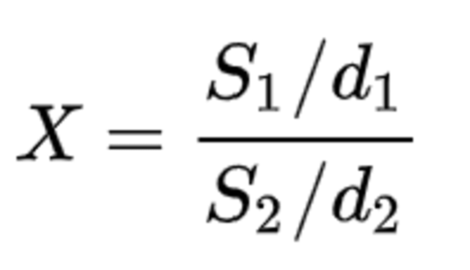
The distribution of the ratio Х is called F-distribution with d1 and d2 degrees of freedom (> 0). 

The two degrees of freedom determine the shape of the distribution. The F-curve is non-symmetrical and is often right-skewed and starts at 0 on the horizontal axis and extends indefinitely to the right, approaching, but never touching the horizontal axis. When the degrees of freedom on the numerator are increased, the right-skewness is decreased.

Below you can see the graph of an F-distribution for different values of degree of freedom d1 and d2:

The PDF for F-distribution is:

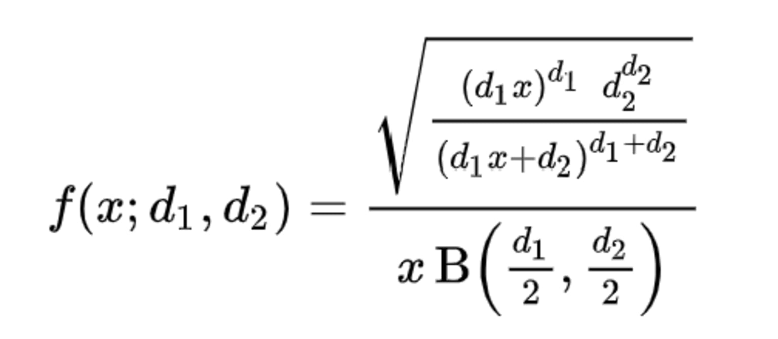
Where f(x;d1, d2) is the probability density function of F-distribution, x > 0, B is the Beta function, and the two parameters d1 and d2 which are positive integers.

Beta distribution models random variables with values falling inside a finite interval. The standard beta distribution usually uses the interval [0, 1] – other intervals are also possible – parameterized by two shape parameters, denoted by alpha (α) and beta (β), that appear as exponents of the random variable and control the shape of the distribution. These two parameters must be positive.

The beta distribution is closely related to a discrete probability distribution counterpart, the binomial distribution. The binomial distribution models the number of successes x with a specific number of trials while the beta distribution models the likelihood of success along with uncertainty. 

That is, in the binomial distribution, the probability is taken as a parameter whereas, in the beta distribution, the probability is a random variable. The beta distribution has been applied to model the behavior of random variables limited to intervals of finite length in a wide variety of disciplines.

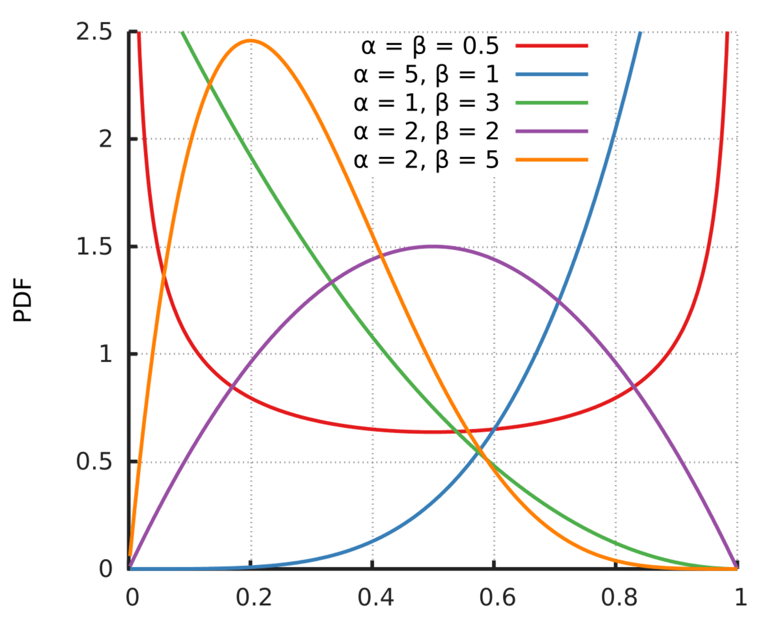
The graph of a Beta distribution looks like this:

The PDF to compute beta distribution is:

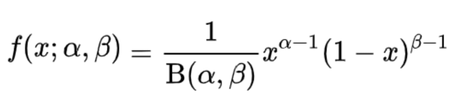
Where f(x;α,β) is the probability density function, Β is the Beta function which acts as a normalizing constant, and α and β are the two positive shape parameters. The beta distribution can take on several shapes including bell-shaped unimodal (when α, β >1), bimodal (when 0 < α, β < 1), and skewed distributions (when one of α or β is less than 1 while the other is greater than 1).

An intuitive example where the beta distribution comes in handy pertains to the batting averages of baseball players. The batting average is a statistic that measures the performance of batters.

The beta distribution is best suited because it allows us to represent prior expectations about most batting averages. That is, in the case where we don't know what a probability is in advance, but we have some reasonable guesses. Through beta distribution, we can represent what we can roughly expect a player's batting average to be before his first swing.

The Weibull distribution is another two-parameter distribution that depends on scale (λ) and shape (k), both > 0. Depending on the value these parameters take, it resembles a normal distribution or asymmetric distribution, such as the exponential distribution. It is often used for statistical modeling of wind speeds or for describing the durability and failure frequency of electronic components or materials. 

Unlike an exponential distribution, it takes into account the history of an object, has memory, and takes into account the aging of a component not only over time but depending on its use. It can be adapted to rising, constant, and falling failure rates of technical systems.

The graph of a Weibull distribution looks like this:

The PDF to compute Weibull distribution is:

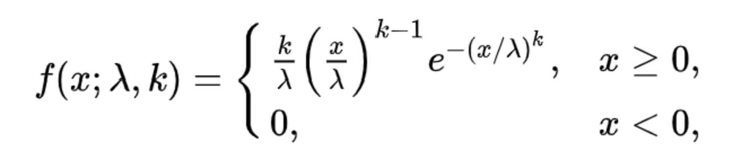
Where f(x;λ,k) is the probability density function of the Weibull distribution, k is the shape parameter and λ is the scale parameter. 

If λ increases, while k is kept the same, the distribution gets stretched out to the right, and its height decreases while maintaining its shape. If λ decreases, while k is kept the same, the distribution gets pushed in towards the left (i.e., towards its beginning or towards 0), and its height increases. If the value of λ is kept the same while the value k=1, it leads to the exponential distribution. If the value of k1 then it has a density that approaches 0 as x approaches 1.

We've seen the importance of knowing what probability distribution your data follows before conducting any statistical tests and have gone through 8 common continuous probability distribution types.

You can read about how you can automatically identify your data's distribution using KNIME Analytics Platform, an open-source, low-code/no-code software, in the blog post: Identify Continuous Probability Distributions with KNIME

Download the Continuous Probability workflow from the Statistics with KNIME space on the Hub and try it out yourself. It's free.