
Deep Learning is the modern revolution of classical neural networks including enhanced and deeper network architectures, as well as improved algorithms for training [deep] neural networks. This blog post introduces you to the basics behind [deep] neural networks, how they are trained, and how you can define, train, and apply [deep] neural networks in a code-free way.
So let’s start with the basics of neural networks to understand the idea behind deep neural networks, before showing you how deep learning is applied in KNIME Analytics Platform. If you already know the basics and want to find out how deep learning is done in KNIME, you can jump to Deep Learning in KNIME Analytics Platform section further down the page.
From a Single Neuron to a Feed Forward Neural Network
The smallest and simplest neural network (strictly not a network yet) is a single artificial neuron. It is the smallest building block in every [deep] neural network.
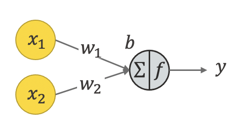
A single artificial neuron is loosely inspired by a biological neuron. It has some inputs (x1and x2 in Figure 1), which are used to calculate the output using some fixed weights w1, w2, a bias b, and a defined activation function f. To calculate the output two steps are performed.
Step 1: Each input is multiplied by the associated weight. Then the sum of all terms plus the bias is calculated
x1* w1+x2*w2 +b
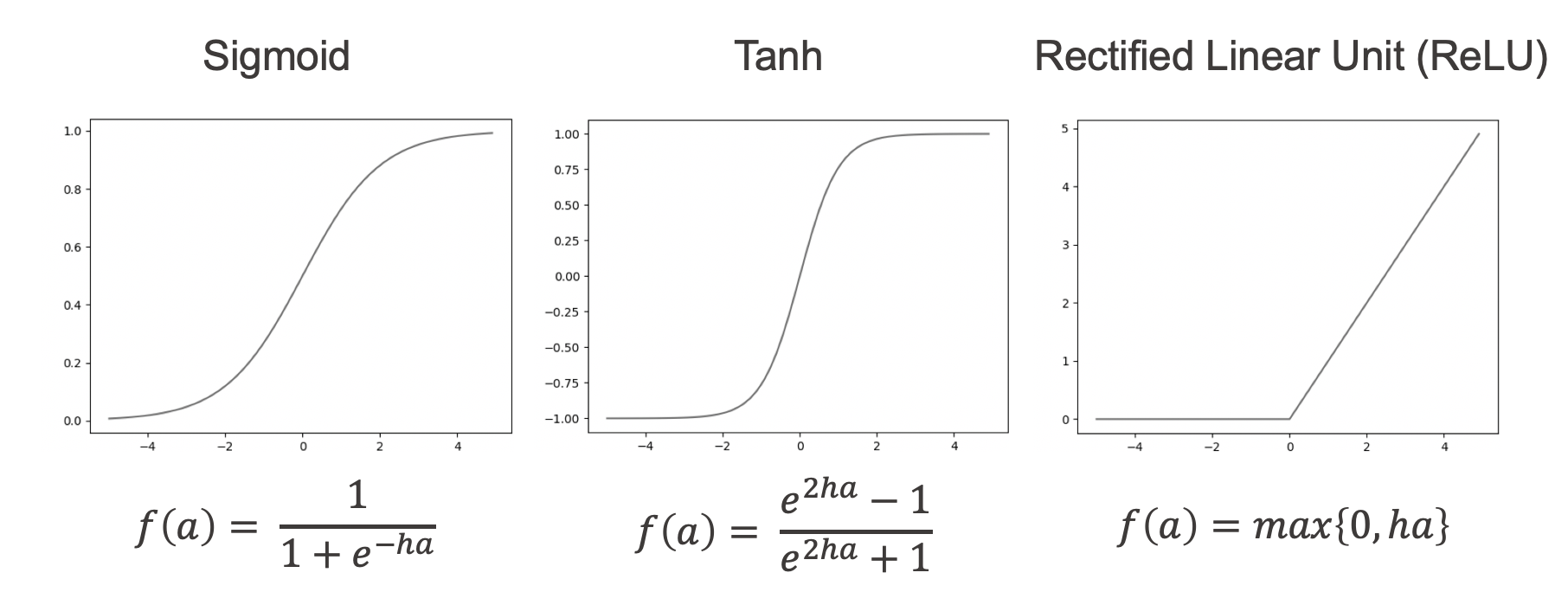
Step 2: An activation function f e.g., sigmoid, tanh, or ReLU, converts the result into the neuron output.
o= f(x1* w1+x2*w2 +x3*w3 +b)
The choice of the activation function is one of the design questions when defining a [deep] neural network. Figure 2 shows some commonly used activation functions. The output of the sigmoid function, for example, is always between 0 and 1. This allows us to interpret the output as the probability of a class. Therefore it is commonly used in the network output layer for binary classification problems.
In a [deep] neural network many artificial neurons are combined into a network. An example of how to connect them is shown in Figure 3. This is called a fully connected feedforward neural network or multilayer perceptron.
Each neuron has its own set of weights and a bias. For simplicity the weights and bias values are not shown in Figure 3. All neurons in the same layer usually use the same activation function.
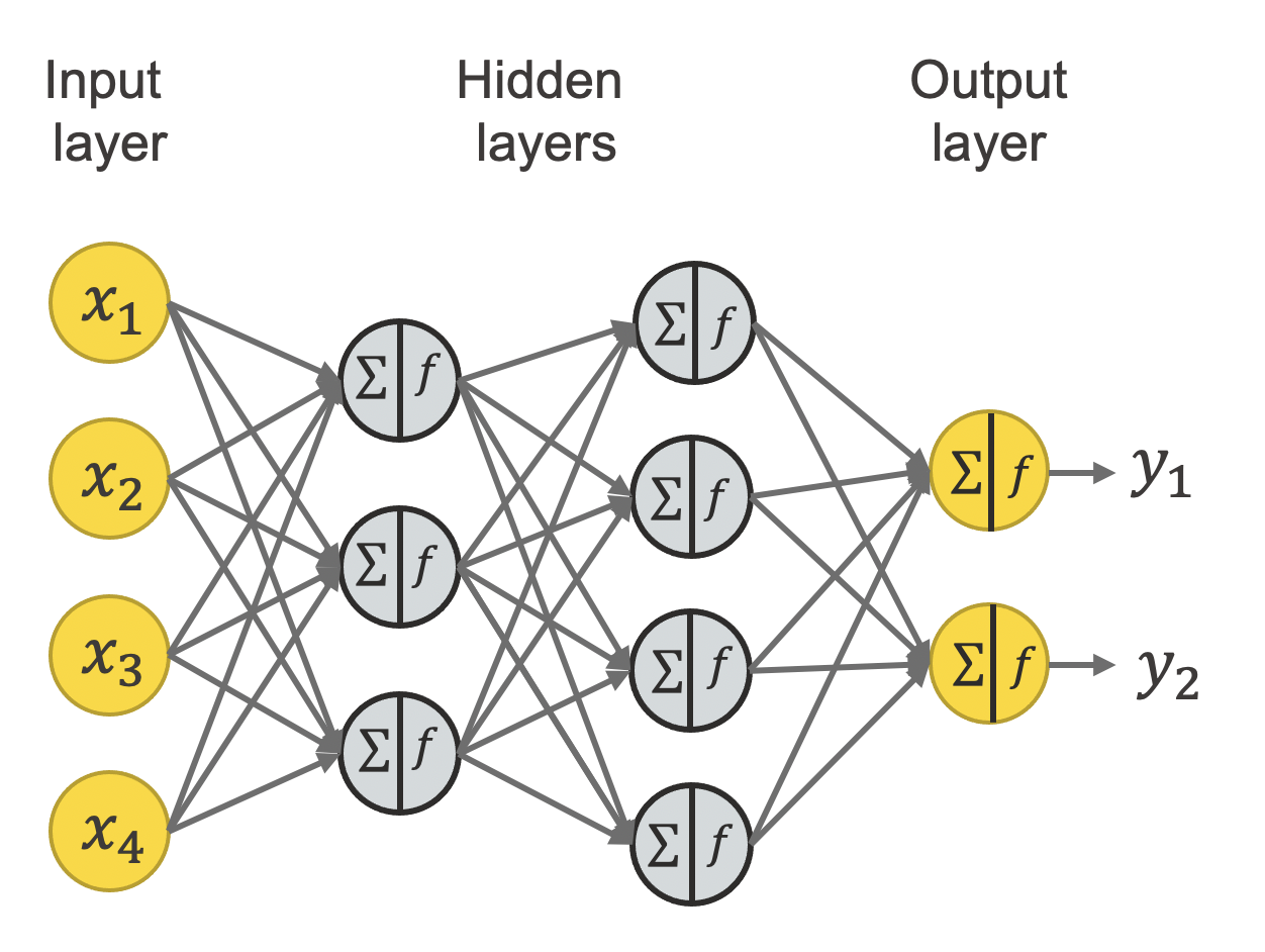
The network in figure 3 starts with the input layer on the left. This layer defines the number of inputs of the network and doesn’t perform any calculation. This is followed by two hidden layers. The first hidden layer uses the input values to calculate the output of its three neurons, by performing the two steps mentioned above for each neuron. The second hidden layer uses the outputs of the first hidden layer to calculate the output of its four neurons. Finally, the output layer uses these values as input to calculate its outputs.
Feedforward neural networks (FFNN) can be used for many tasks. The most common tasks are classification and regression. A special task is anomaly detection. In this case we use a special FFNN architecture, named autoencoder. Learn more about autoencoders in this post Fraud Detection using Random Forest, Neural Autoencoder, and Isolation Forest techniques.
Feedforward neural networks (FFNN) can be used for many tasks. The most common tasks are classification and regression. A special task is anomaly detection. In this case we use a special FFNN architecture, named autoencoder. Learn more about autoencoders in this post Fraud Detection using Random Forest, Neural Autoencoder, and Isolation Forest techniques.
Summarizing, in a fully connected feedforward neural network information travels from the input layer to the output layer, without any loop or backward connections. It is called fully connected as each neuron of the previous layer is connected to all neurons in the next layer. This layer type is called a dense layer.
More hidden layers with different numbers of neurons and different activation functions can be added to the network for more complexity, which makes it deeper.
From a Feedforward Neural Network to Deep Learning
To cover all kinds of use cases and data formats, like images or sequential data, many different layer types and architectures have been developed by deep learning researchers. A detailed introduction to these layers and architectures are topics for further blog posts.
Popular deep learning architectures are:
- Convolution Neural Networks (CNN) are especially popular when it comes to image data and computer vision tasks. Typically in a CNN multiple convolutional and pooling layers are used to extract a hierarchy of features in images. The blog post Introduction to Convolutional Neural Networks and Computer Vision gives you a short introduction.
- Recurrent Neural Networks (RNN) are commonly used for sequential data, e.g. time series data or text. The key idea is a loop connection in the network, which allows the network to remember information from the previous values in the sequence. Popular recurrent layers are GRU layer and LSTM layer. The blog post "Once Upon A Time … “ by LSTM Network gives you a short introduction to RNNs.
Once the network architecture is defined the next step is to train the network.
Training a [Deep] Neural Network
Training a [deep] neural network means estimating the weights for all neurons that lead to the correct predictions. The training procedure starts with random weights and applies the network to the training set. Then a loss function is used to measure the error between the predicted value and the expected outcome. Based on this loss function, the weights in the network are updated using some flavour of gradient descent with an efficient way of calculating the gradient, called back propagation. Afterwards the network with the new weights is again applied to the training set and the procedure is repeated until we have a set of good weights.
Research papers and use case specific blog posts are great resources to get inspiration for your own use case. Many different flavors of gradient descent have been developed by researchers, called optimizers. The blog post An overview of gradient descent optimization algorithms by Sebastian Ruder gives an overview of different optimizers.
The choice of the loss function is another design choice and depends on the problem at hand. Below are some tips for the settings of the last layer of a [deep] neural network and the loss function.
In summary: to train a [deep] neural network we need to define:
- A network architecture, fitting the use case and data type
- A loss function, fitting the use case and network architecture
- An optimizer for the training
Implementing Deep Learning Models
There are many open source frameworks that allow you to define and train [deep] neural networks. One of them is TensorFlow developed by Google Brain. A more user-friendly interface for TensorFlow is the open source library Keras, which still requires you to code. The Keras Integration of KNIME Analytics Platform adds an even more user-friendlier interface on top, borrowing the graphical interface of KNIME Analytics Platform to define, train, and apply deep learning models.
Let’s see how we can define, train, and apply a [deep] neural network in KNIME data analytics platform. As an example, we have chosen an image classification task, based on the MNIST fashion dataset. Input images are 28 x 28 gray-scaled images of clothing articles. The deep neural network used for this task is a Convolutional Neural Network (CNN).
Deep Learning in KNIME Analytics Platform
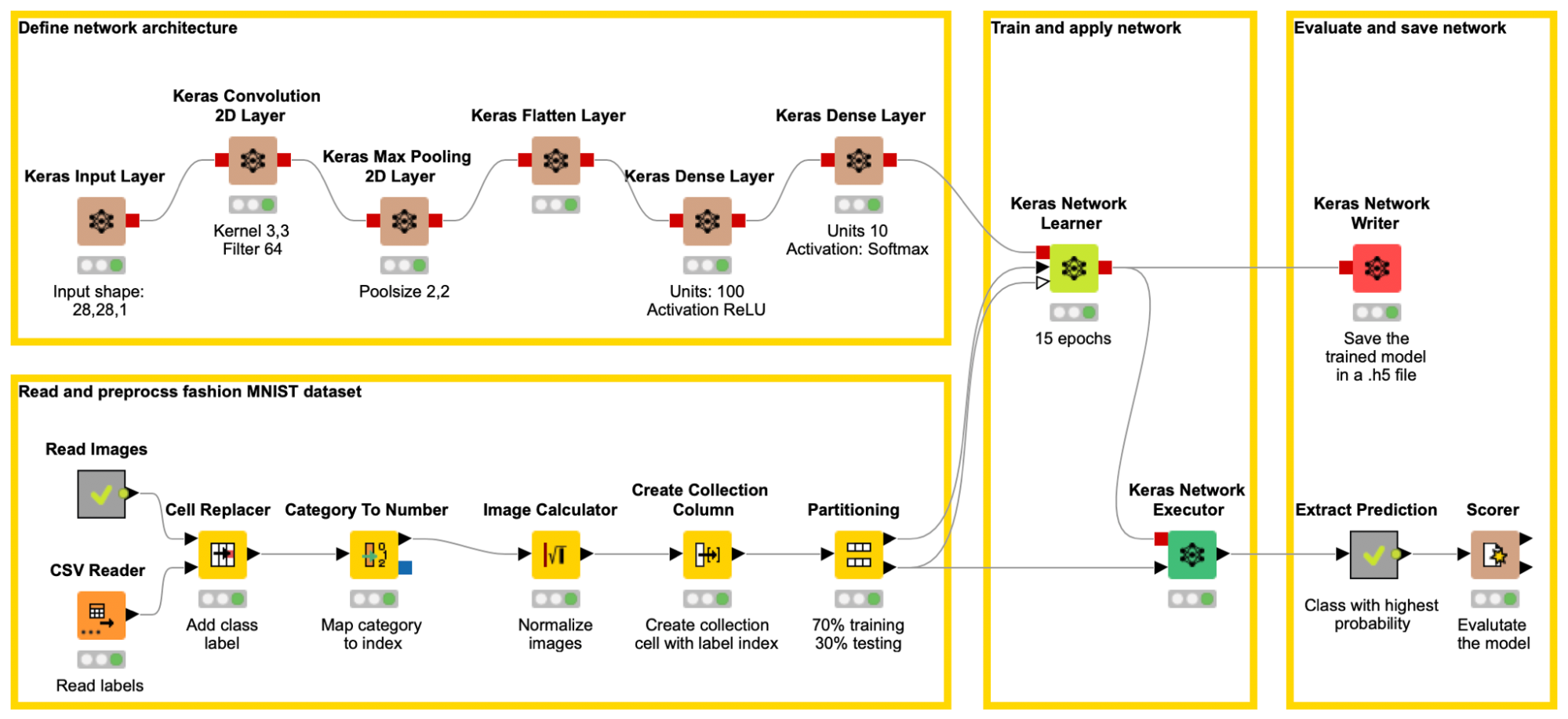
The example workflow CNN for Image Classification of the MNIST Fashion Dataset, below (figure 4) covers all steps of any deep learning project, CNN, or any other type of network: From reading data through to applying the trained network to test data, using the KNIME Keras Integration.
Step 1: Define the Network Architecture
The KNIME Deep Learning - Keras Integration comes with a set of layer nodes, each implementing another layer type. Here are just a few:
- Keras Input Layer node to define the input,
- Keras Dense Layer node to define fully connected layers,
- Keras Convolutional 2D Layer node for CNNs,
- Keras LSTM Layer node for RNNs,
Each node comes with a configuration window that allows you to define all necessary settings in a layer e.g., the number of neurons (called units in Keras) or the activation function.
Via drag and drop these nodes can be added and connected to define the network architecture. For the MNIST Fashion example a shallow CNN is built in the upper left part of the workflow (brown nodes), with 6 neural layers including the input layer. (See the appendix for a detailed description of the defined network architecture).
A dense layer with activation softmax and as many units as different classes is commonly used as the output layer for a multiclass classification. It allows us to interpret the output as the probability of the different classes. For that, the different class labels must be encoded as one-hot vectors, during training.
Step 2: Read and Preprocess the Data
The lower left part of the workflow reads the gray-scaled images of the MINST fashion dataset, adds the label information, performs preprocessing steps like normalizing the images, mapping each label to an index, and partitioning the data into a training and a test set. Below (figure 5), you can see a subset of the dataset including a column with the index encoded labels.
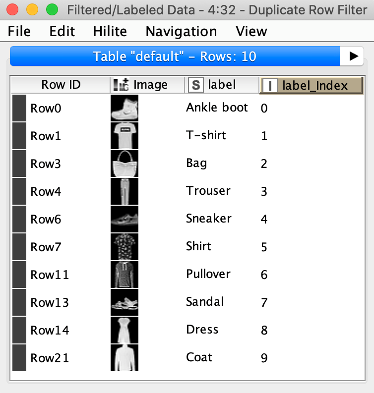
The Create Collection Column node converts the label index into a collection cell. This allows the Keras Network Learner node to convert the index values into one-hot-vectors during training.
Step 3: Train the Deep Learning Model
In the configuration window you define the loss function; the columns with the input for the network (here, the image); the target column (here, the collection cell with index encoded class label); the training settings e.g., epochs, batch size, optimizer.
During execution the training progress can be monitored via the interactive learning monitor view. It shows the progress of the accuracy and the loss over the different epochs.
Explanation of the different training settings.
- Epochs: Number of times the training dataset is passed through the network to update the weights. In the example the network was trained for 20 epochs.
- Batch size: Usually not the whole dataset is used to update the weights. The batch size defines how many rows are used for each weight update. In this example a batch size of 32 is used.
Step 4: Apply and Save the Trained Deep Learning Model
The example workflow - CNN for Image Classification of the MNIST Fashion Dataset - above, in figure 4 uses the introduced nodes to train the defined network architecture, to apply the trained network to the test set, and to save it. Afterwards the class with the highest probability is extracted and the model is evaluated. With the defined network and training parameters the deep learning model reaches an accuracy of 91%.
Want to try it out? Download the example workflow CNN for Image Classification of the MNIST Fashion Dataset publicly available on the KNIME Hub.
Appendix
Here is a more detailed description of the network architecture that was defined in Figure 4.
- The Keras Input Layer node that defines the input shape of the network. In this example the input shape is 28,28,1 as the gray-scaled images are of size 28 x 28 pixels and only one value is used to represent the shade of gray of each pixel, aka only one channel.
- A Keras Convolutional 2D Layer node with 64 filters of size 3 x 3. This means the network learns to check for 64 different features of size 3x3 in the images. This can be edges, corners etc.
- A Keras Max Pooling 2D Layer node which replaces every 2 x 2 area of the output of the previous layer with the maximum value.
- A Flatten Layer node that converts the matrix into a vector.
- A Keras Dense Layer node with 100 units and activation ReLU as hidden layer.
- A Keras Dense Layer node with 10 units and activation softmax as output layer.
Set up Keras in KNIME Analytics Platform
If you would like to try out the workflow in this article, you will need the KNIME Deep Learning - Keras Integration. This builds onto the KNIME Python Integration. You’ll find the installation instructions to set it up in the KNIME Deep Learning Integration Installation Guide.