
Microbiomes live inside us and on us and are real multi-taskers. They break down nutrients that our body couldn’t break down by itself. They train our immune system. And they are first in line in our defense against pathogens. Our health depends on them.
The analysis of the quality and quantity of microbiomes is therefore an important undertaking. This article takes a look at one of the steps involved in this analysis called taxonomic profiling. Taxonomic profiling determines where exactly a group, or community, of microbes is living in or on the body - for example the gut - and then estimates how many of them there are.
The Human Gut
The human gut is home to a lot of bacteria (approx. 10^9!) plus other microorganisms we collectively call microbes.These microbes play a wide range of roles in keeping us healthy. And in order for them to keep us healthy and for us to - well - provide for them, there needs to be a particular composition of different types (species) of microbes so that we get key nutrients in the right amounts.. Diseases like Irritable Bowel Syndrome (IBS) and Inflammatory Bowel Disease (IBD) 2 4 5 are the result when this mix is sub-optimal.
Researchers have been looking at different treatment strategies (probiotics, prebiotics, symbiotics and antibiotics 5 8) to alter microbiome composition to achieve a state that promotes gut health. While these strategies are still in need of formation to become standard treatment, fecal transplant from a healthy donor to a patient with IBD is gaining momentum as an alternative and blanket solution. The ultimate goal: to replace the gut microbial community of the patient with that of the healthy donor.
DNA Sequencing
In order to evaluate whether or not the transplant works, the composition of the gut microbial community needs to be monitored before and after the transplant, for example by taking environmental samples, extracting the genetic material, and performing DNA sequencing. The resulting data enables us to infer which types of organisms are in the sample and the prevalence of each type. This is done by using the subtle differences in nucleotide sequences among genomes/genes of different bacterial species. In this article, I focus on using a particular gene, namely the 16S ribosomal RNA gene, for this purpose.
Analysis of 16S-rRNA Data
This blog presents a KNIME workflow that has been created to analyze 16S-rRNA data obtained from the gut of 10 IBD patients at different time points while they undergo fecal transplants. The overall goal is to understand the shift in gut microbiome composition with the help of multiple visualizations. Using an interactive sunburst chart (below), I can visualize which group of bacteria are common and show how prevalent they are in the human gut. Being interactive, users can click on portions of the chart to display the actual sequences that are tied to the selected group and see their count in a table view.
The workflow ultimately produces a JavaScript visualization, which shows the shift in microbial composition of individual patients via a dashboard of stacked bar plots. This visualization makes it very easy to compare the microbial composition of the donor’s gut with the gut microbiome of the receiver at different time points.
The full article showcases how to get the data from the European Nucleotide Archive via REST and FTP services, how to preprocess the data, use an external R-package within KNIME, and visualize multiple microbiome composition so as to compare them. The integration of complex and domain specific external R packages in KNIME enables the creation of workflows that are not just transparent and easy to understand, but also sufficiently powerful to get the job done.
Additional use cases for this workflow
The workflow can be used for analysing microbial communities from any other sources. The use cases could range from soil microbiome analysis to monitor the fertility of a soil to environmental bioremediation where microorganisms are used to clean up environmental messes such as oil spills.
Read the full blog article here:
Abstract
Microbiomes living inside and on us produce essential enzymes, breakdown nutrients that our body by itself couldn’t, train our immune system and are our first line of defense against pathogens. Our health depends on them. This makes qualitative and quantitative analysis of microbiomes an important undertaking. The first step of such analysis is to know which group of microbes are living in a particular body site, such as our gut, and to estimate their respective relative abundances. This step is known as taxonomic profiling. In this blog, I present a step by step guide how to perform taxonomic profiling on microbial communities using the 16S ribosomal RNA gene as a fingerprint. The data I picked is coming from a study on the dynamics of the gut microbiome during the process of fecal transplant in 10 inflammatory bowel disease (IBD) patients. 16S-rRNA sequences were collected from fecal samples of IBD patients and their donors at different time points of fecal transplant. I will be using the KNIME Analytics Platform and its R-Integration for the whole process. The R-Integration of KNIME allows me to use a domain specific program called DADA2 which is available only as an R package. The blog showcases how to get data directly from the European Nucleotide Archive (https://www.ebi.ac.uk/ena) via REST and FTP services, pre-process data, use an external R-package within KNIME Analytics Platform, and visualize multiple microbiome composition with the purpose of comparing them.
Human Gut Microbiome
The human gut, irrespective of its health state, is home to approximately 10^9 bacteria and other microorganisms which we collectively refer to as microbes. These microbes are of various sorts and play a wide range of roles in keeping us healthy. But for this (them keeping us healthy and we, well, providing for them) to work, there needs to be a particular composition of different types (species) of microbes. Only then, we can get the essential nutrients just in the right amount, for example. Not having a “good configuration” of the gut microbiome, in other words gut dysbiosis, can cause diseases like Irritable Bowel Syndrome (IBS) and Inflammatory Bowel Disease (IBD) 2 4 5.
Researchers have been looking at different treatment strategies to alter the microbiome composition towards a state that promotes gut health. The strategies include probiotics, prebiotics, symbiotics and antibiotics 5 8. While these strategies are still in need of formation to become standard treatment, fecal transplant from a healthy donor to a patient with IBD is gaining momentum as an alternative and blanket solution. The ultimate goal, here, is replacing the gut microbial community of the patient with that of the healthy donor.
To evaluate if the transplant worked or not, one needs to monitor the composition of the gut microbial community before and after transplant. One way of doing that is to take environmental samples, extract all the genetic material from the samples, perform DNA sequencing and use the resulting data to infer
1) which types of organisms are in the sample and
2) what is the prevalence of each type.
This is done by using the subtle differences in nucleotide sequences among genomes/genes of different bacterial species. In this blog post, I will focus on using a particular gene, namely the 16S ribosomal RNA gene, for this purpose.
The 16S ribosomal RNA (16S rRNA) gene
The 16S rRNA gene has the advantage of being highly conserved across almost all prokaryotic species, which facilitates designing primers that can bind to a specific region within the gene 3. The primers are used to selectively perform PCR (Polymerase chain reaction) which produces multiple copies of (parts of) 16S-gene. The resulting sequences are called amplicon sequences. The 16S gene also contains hypervariable regions that can be used as fingerprints to identify the types of bacteria. These variable regions are numbered V1-V9 and have a well-defined locus within the stretch of the gene. In order to identify microbial species/groups, one can use either the entire length of the 16S gene spanning all the variable regions, or part of the 16S gene covering two or three hypervariable regions.
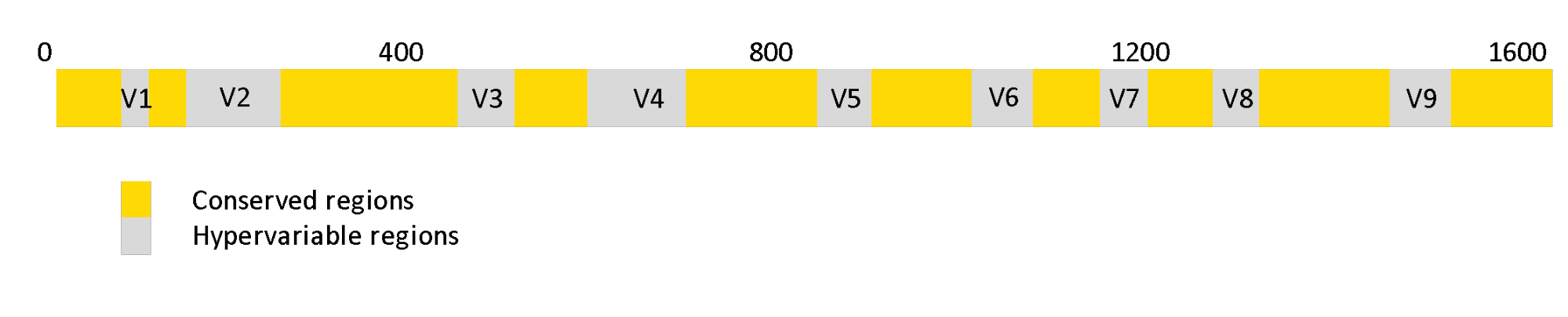
Figure 1. Regions of 16s rRNA genes. The grey regions indicate hypervariable regions that can be used as fingerprints to identify the types of bacteria.
A KNIME Workflow for Gut Microbiome Analysis of IBD Patients from 16S sequencing data
In this blog post, I present a KNIME workflow created to analyze 16S-rRNA data obtained from the gut of 10 IBD patients at different time points while they undergo fecal transplants. The overall goal is to understand the shift in gut microbiome composition with the help of multiple visualizations.
The workflow uses the DADA2 R package by Callahan et al. 1 to determine the microbial composition from the 16S sequences. This is done via the R-Integration of KNIME which allows usage of such domain specific applications available as R packages with minimal effort. Such packages are focussed on solving a particular scientific problem and are results of months of research and being able to use them directly in a KNIME workflow is just great.
A system wide installation of the DADA2 R package is needed for the workflow to work. Installation instructions can be found here. The main result of DADA2 is a table containing a list of unique amplicon sequences called Amplicon Sequence Variants (ASV) and their count. In the workflow, this result will go through further analysis steps using KNIME Analytics Platform to have a dashboard of visualizations of taxonomic profiles across patients and timepoints.

Figure 2. A KNIME workflow for gut microbiome analysis of IBD patients from 16S sequencing data. It can be accessed and downloaded from the KNIME Hub.
In short the workflow does the following:
- Downloads 16S amplicon sequencing files (FASTQ format) from European Nucleotide Archive (ENA)
- Uses the R package DADA2 to quality check the sequences and create an amplicon sequence variant table and assign them to a group of bacteria
- Create taxonomic profile at a desired taxonomic rank
- Visualize the results to demonstrate the change in the composition of gut microbiota of each patients
Let us dive into each step of the workflow and explain the main ideas behind each part/component of the workflow.
- Download the workflow Gut Microbiome Analysis of IBD Patients (16S) from the KNIME Hub.
1. Download FASTQ sequences from ENA
The first thing to do is getting the DNA sequencing data from European Nucleotide Archive (ENA) where it is publicly available under project identifier PRJDB4959. More metadata about the project can be accessed here. I used “Download FASTQ files from ENA” component available from the KNIME Hub to easily retrieve our example dataset from the source. The dataset contains a total of 40 FASTQ files representing 10 donors and 10 patients at 3 different time points after going through fecal microbiota transplantation. In each FASTQ file there are thousands of short DNA sequences (sequencing reads) obtained via amplicon sequencing. The component outputs a table that contains the path to the sequence files of each sample that are downloaded and stored locally (see the table below).
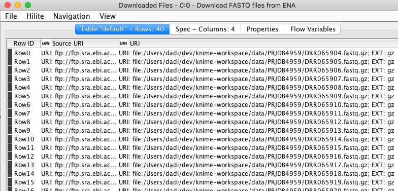
Figure 3. The output of “Download FASTQ sequences” component showing a partial list of sequences downloaded from EBI.
2. Create an Amplicon Sequence Variant (ASV) table
Since I have our sequencing reads of each sample as individual FASTQ files, I can now go ahead and start the analysis with DADA2. A typical DADA2 pipeline starts by inspecting the quality profiles of the input sequencing reads. The results are then used as a guide to perform error correction on the original sequences to account for sequencing errors. Then sequences are truncated at a length where the quality drops for the majority of the sequences. The details on how exactly this is done can be found in the DADA2 paper (Callahan et al.) and I leave that to the interested reader. The error correction is followed by a series of R Scripting nodes matching each stage of the DADA2 pipeline. Each node mostly performs a singular task by calling a DADA2 routine/function. Here is an example code snippet inside the R to R node that filter sequences.
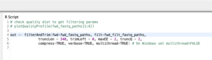
Figure 4. An example R code snippet that filters and trims sequences
It is of course possible to use just a single R to R node with the combined R source code instead of a series of nodes. But, I think the later representation makes both understanding and maintaining the pipeline easier.
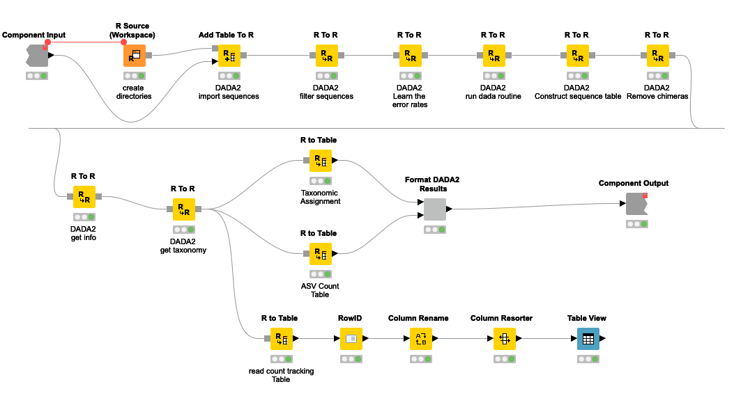
Figure 5. DADA2 pipeline represented by a series of KNIME R Scripting nodes.
The pipeline can be summarized into 5 steps.
- Sequences below a certain threshold length and quality are filtered out
- By looking at the error profile, noisy sequences are filtered out. Here probabilistic error correction is done to account for nucleotide differences that are artifacts of the sequencing process.
- A table of ASVs and their frequency in each sample is generated.
- Chimeric sequences are removed. Chimeric sequences are sequences that do not exist naturally but created by a faulty PCR process in which sequences from two different origins are artificially concatenated.
- After getting the ASV count table, the next step is to decode each ASV into a (group of) bacteria/taxa known to be associated with it. I will use a database curated and provided by the authors of DADA2. The database contains a list of known amplicon sequences and the taxa they belong to. Ambiguous sequences are assigned to a more generic taxa. For example, 16S sequences that are equally similar between that of species_1 and species_2 will be assigned to a group that covers both species. In this process a given ASV can be assigned to a single bacterial species or at a higher level of taxonomy such as genus or family. This is dependent on the specificity of the ASV.
At the end I will have two tables:
a) An ASV table where different variants of 16S sequence fragments are represented as rows and samples are represented by columns. The values in the table represent how often a sequence (row) is observed in a sample (column).
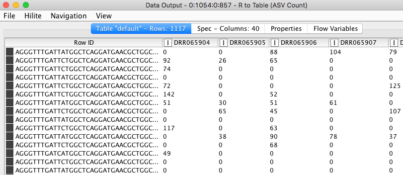
Figure 6. ASV count table. Values in the table show the frequencies of each amplicon sequence variant (rows) in different samples (columns).
b) The assignment of individual ASVs to a taxonomic entry.
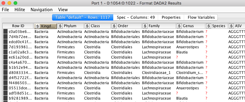
Figure 7. Assignment of individual ASVs to a taxonomic entry.
Quality control
Before proceeding into joining tables, aggregating and visualizing the results, one needs to check how many of the original sequencing reads made it through each stage of the analysis per sample. There is a dedicated functionality of the DADA2 package for this purpose. I exposed the result through the Table View node, where the number of sequencing reads that were available originally and how many of them passed different filtration steps are shown. One should look out for an unreasonable reduction of read count, as that could mean a bad sample or wrong combination of parameters in the pipeline.
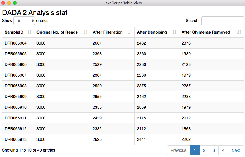
Figure 8. Sequencing read statistics. The quality looks good, as there is no unreasonable reduction of read count.
The table containing the analysis statistics looks just fine. Starting from 3000 sequencing reads I ended up with 2376, 1989, and 2123 reads. For the second row the chimera removal step took away about 300 reads which is quite higher compared to the other two displayed here. Chimeric sequences are simply sequences that do not exist naturally but created by a faulty PCR process in which sequences from two different origins are artificially concatenated.
3. Create taxonomic profile at a desired taxonomic rank
Depending on the level granularity required or for the purpose of finding more fitting patterns among samples or sample groups it is important to produce taxonomic profiles at different relative levels of grouping (taxonomic ranks). In the workflow, it is possible to select among 7 different ranks. The ranks are Kingdom, Phylum, Class, Order, Family, Genus and Species from generic to specific. Selecting the rank is usually done by looking at the taxonomic assignment and the most specific rank with not too many missing values in the corresponding column is chosen. In our example, this is either genus or family. The counts of sequences will be grouped by the chosen rank and relative abundance is calculated to show the percentage of each group of that taxonomic rank.
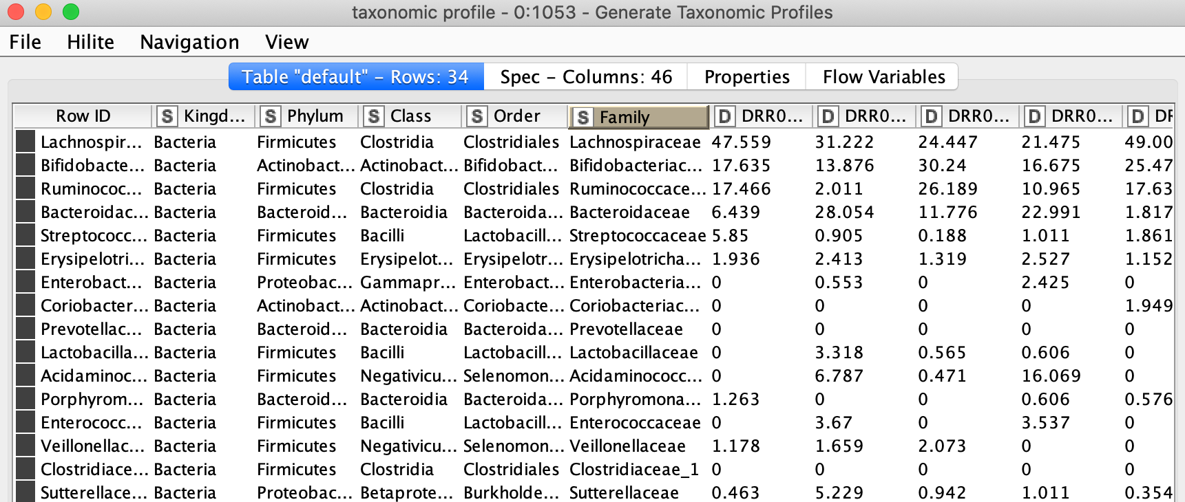
Figure 9. Relative abundance table at family level of the taxonomy
4. Visualize the results
It is natural to ask which types of Bacteria are found in a human gut. Using an interactive sunburst chart, I can visualise which group of bacteria are common and their prevalence in the human gut (see Figure 10). The charts represent aggregated/averaged relative abundance of bacterial groups at different taxonomic levels from healthy donors (left) and IBD patients before a fecal transplant (right). Clicking on each portion of the charts displays the actual of sequences that are tied to the selected group and their count in a table view.
A simple BLAST of the sequences on NCBI can verify the sanity of the method by checking if the sequences are actually related to the group they are assigned to by the pipeline. If you want to learn more about BLAST and do BLASTing without leaving your KNIME Analytics Platform, check out the BLAST from the PAST blog post by Jeany Prinz.
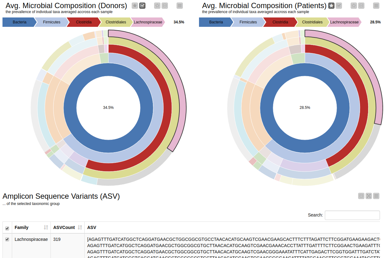
Figure 10. Sunburst charts showing the average composition of the gut microbiome in healthy donors (left) and IBD patients before transplant (right). Selecting a group will show the corresponding sequences representing that group of bacteria in the samples.
The commensal (more common) bacterial families are Lachnospiraceae, Bifidobacteriaceae, Ruminococcaceae and Bacteroidaceae. In general, these groups are higher in abundance in the healthy patients. If we take the currently selected group Lachnospiraceae for example, it is higher in the donors than in patients. These observations are in-line with literature which suggests that IBD patients are characterized by a lower abundance of Bacteroidetes and Lachnospiraceae compared to healthy controls 4.
The final step of our workflow produces a JavaScript visualization whereby the shift in microbial composition of individual patients is represented as a dashboard of stacked bar plots. The right most stacked bar is always the microbial composition of the donor’s gut, whereas the other three bars to the right represent the gut microbiome of the receiver at different time points.
First of all, it is interesting to note that the composition of gut microbiomes differ among individuals. This is true even in the healthy donors. Secondly, the patients’ gut microbiomes showed some changes towards those of the donors’, although in some cases, these changes didn’t persist overtime for all patients. For example, the bacterial family Ruminococcaceae (Orange) was present in high abundance in the donor's gut but not so in patient A. But after a week from the transplant it also became as abundant in the patient. Similarly, in patient D the proportion of the bacterial families Streptococcaceae (green) and Enterobacteriaceae (red) were absent in the beginning. But after a week from the transplant these groups of bacteria cover a large proportion of the patient’s gut microbiome, as they did in the patient's respective donor.
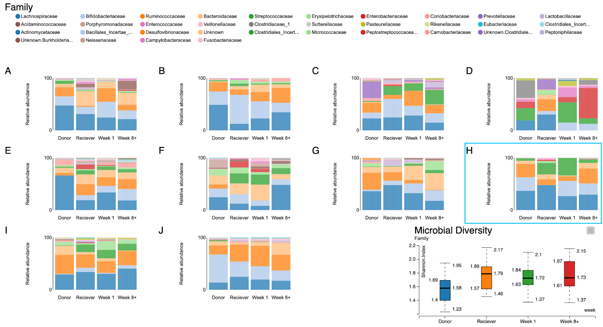
Figure 11. A dashboard of visualizations of taxonomic profiles across 10 patients + their donors (A-J) through different timepoints.
Let us take a closer look at patient H. From the bar plot it is clear that in the beginning patient H has close to zero Bifidobacteriaceae family in his gut. On the contrary the Donor has an abundance of the same family of bacteria. After the fecal transplant it can be seen that the abundance of this group of bacteria increased significantly. And it is known from literature [6,7] that probiotics rich in Bifidobacteria are successfully used in treating patients with inflammatory bowel diseases.
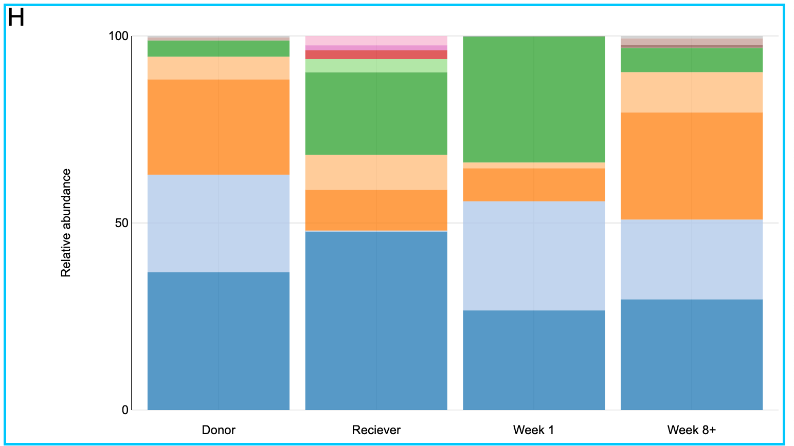
Figure 12, a closer look at the taxonomic profiles of patient J and his/her donor
Side Note
I can not confirm if the patient's health has improved due to the fecal transplant since I don't have the full treatment data available. I only have the sequencing data with the patient ID and time points at our disposal. It is also unclear if these positive changes are long lasting as the study is limited to 8-12 weeks. I am also fully aware that this is not even close to enough for making scientific conclusions. The focus here is to demonstrate how a KNIME workflow can be developed and used to assist a comparative study of microbial communities at different time points.
Summary
We have created a KNIME workflow that retrieves sequencing data from public repositories, analyses them, and creates useful visualisations to investigate the changes in microbial composition of patients' gut. We have learned how we can use 16S rRNA amplicon sequences for characterisation of microbial communities in KNIME Analytics Platform. Most importantly, we showed how we can integrate complex and domain specific external R packages in KNIME to create workflows that are transparent and easy to understand but yet powerful enough to get the job done.
The workflow can be used for analysing microbial communities from any other sources. The use cases could range from soil microbiome analysis to monitor the fertility of a soil to environmental bioremediation where microorganisms are used to clean up environmental messes such as oil spills.
References
1. Callahan BJ, McMurdie PJ, Rosen MJ, Han AW, Johnson AJ, Holmes SP. DADA2: High-resolution sample inference from Illumina amplicon data. Nat Methods. 2016;13(7):581–583. doi:10.1038/nmeth.3869
2. Ruairi Robertson,, 'Why the Gut Microbiome Is Crucial for Your Health', www.healthline.com, June 27, 2017, accessed Feb 2020, https://www.healthline.com/nutrition/gut-microbiome-and-health
3. Wang, Y., & Qian, P. Y. (2009). Conservative fragments in bacterial 16S rRNA genes and primer design for 16S ribosomal DNA amplicons in metagenomic studies. PLoS ONE, 4(10). https://doi.org/10.1371/journal.pone.0007401
4. Kennedy PJ, Cryan JF, Dinan TG, Clarke G. Irritable bowel syndrome: a microbiome-gut-brain axis disorder?. World J Gastroenterol. 2014;20(39):14105–14125. doi:10.3748/wjg.v20.i39.14105
5. Distrutti E, Monaldi L, Ricci P, Fiorucci S. Gut microbiota role in irritable bowel syndrome: New therapeutic strategies. World J Gastroenterol. 2016;22(7):2219–2241. doi:10.3748/wjg.v22.i7.2219
6. Halfvarson J, Brislawn CJ, Lamendella R, et al. Dynamics of the human gut microbiome in inflammatory bowel disease. Nat Microbiol. 2017;2:17004. Published 2017 Feb 13. doi:10.1038/nmicrobiol.2017.4
7. Pozuelo M, Panda S, Santiago A, et al. Reduction of butyrate- and methane-producing microorganisms in patients with Irritable Bowel Syndrome. Sci Rep. 2015;5:12693. Published 2015 Aug 4. doi:10.1038/srep12693
8. McFarland LV, Dublin S. Meta-analysis of probiotics for the treatment of irritable bowel syndrome. World J Gastroenterol. 2008;14(17):2650–2661. doi:10.3748/wjg.14.2650