
In this blog series we’ll be experimenting with the most interesting blends of data and tools. Whether it’s mixing traditional sources with modern data lakes, open-source devops on the cloud with protected internal legacy tools, SQL with noSQL, web-wisdom-of-the-crowd with in-house handwritten notes, or IoT sensor data with idle chatting, we’re curious to find out: will they blend? Want to find out what happens when IBM Watson meets Google News, Hadoop Hive meets Excel, R meets Python, or MS Word meets MongoDB?
Today: Blending Databases. A Database Jam Session

The Challenge
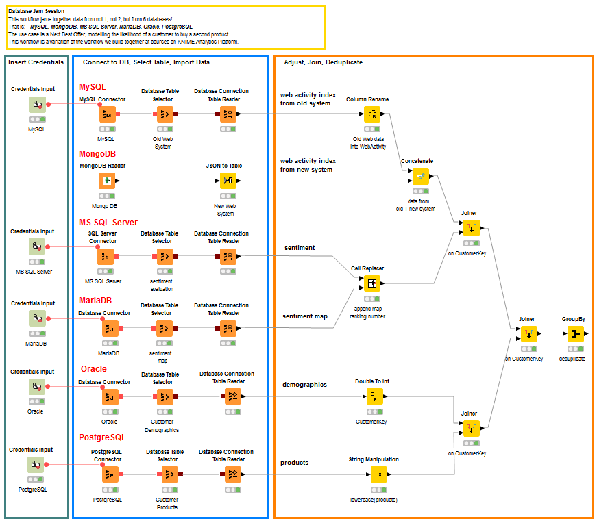
Today we will push the limits by attempting to blend data from not just 2 or 3, but 6 databases!
These 6 SQL and noSQL databases are among the top 10 most used databases, as listed in most database comparative web sites (see DB-Engines Ranking, The 10 most popular DB Engines …, Top 5 best databases). Whatever database you are using in your current data science project, there is a very high probability that it will be in our list today. So, keep reading!
What kind of use case is going to need so many databases? Well, actually it’s not an uncommon situation. For this experiment, we borrowed the use case and data sets used in the Basic and Advanced Course on KNIME Analytics Platform. In this use case, a company wants to use past customer data (behavioral, contractual, etc…) to find out which customers are more likely to buy a second product. This use case includes 6 datasets, all related to the same pool of customers.
- Customer Demographics (Oracle). This dataset includes age, gender, and all other classic demographic information about customers, straight from your CRM system. Each customer is identified by a unique customer key. One of the features in this dataset is named “Target” and describes whether the customer, when invited, bought an additional product. 1 = he/she bought the product; 0 = he/she did not buy the product. This dataset has been stored in an Oracle
- Customer Sentiment (MS SQL Server). Customer sentiment about the company has been evaluated with some customer experience software and reported in this dataset. Each customer key is paired with customer appreciation, which ranges on a scale from 1 to 5. This dataset is stored on a Microsoft SQL Server
- Sentiment Mapping (MariaDB). This dataset here contains the full mapping between the appreciation ranking numbers in dataset # 2 and their word descriptions. 1 means “very negative”, 5 means “very positive”, and 2, 3, and 4 cover all nuances in between. For this dataset we have chosen storage relatively new and very popular software: a MariaDB
- Web Activity from the company’s previous web tracking system (MySQL). A summary index of customer activity on the company web site used to be stored in this dataset. The web tracking system associated with this dataset has been declared obsolete and phased out a few weeks ago. This dataset still exists, but is not being updated anymore. A MySQL database was used to store these data.
- Web Activity from the company’s new web tracking system (MongoDB). A few weeks ago the original web tracking system was replaced by a newer system. This new system still tracks customers’ web activity on the company web site and still produces a web activity index for each customer. To store the results, this system relies on a new noSQL database: MongoDB. No migration of the old web activity indices has been attempted, because migrations are costly in terms of money, time, and resources. The idea is that eventually the new system will cover all customers and the old system will be completely abandoned. Till then, though, indices from the new system and indices from the old system will have to be merged together at execution time.
- Customer Products (PostgreSQL). For this experiment, only customers who already bought one product are considered. This dataset contains the one product owned by each customer and it is stored in a PostgreSQL
The goal of this experiment is to retrieve the data from all of these data sources, blend them together, and train a model to predict the likelihood of a customer buying a second product.
The blending challenge of this experiment is indeed an extensive one. We want to collect data from all of the following databases: MySQL, MongoDB, Oracle, MariaDB, MS SQL Server, and PostgreSQL. Six databases in total: five relational databases and one noSQL database.
Will they all blend?
Topic. Next Best Offer (NBO). Predict likelihood of customer to buy a second product.
Challenge. Blend together data from six commonly used, SQL and noSQL databases.
Access Mode. Dedicated connector nodes or generic connector node with JBDC driver.
The Experiment
Let’s start by connecting to all of these databases and retrieving the data we are interested in.
Relational Databases
Data retrieval from all relational SQL-powered databases follows a single pattern:
- Define Credentials.
- Credentials can be defined at the workflow level (right-click the workflow in the KNIME Explorer panel and select Workflow Credentials). Credentials provided this way are encrypted.
- Alternatively, credentials can be defined in the workflow using a Credentials Input node. The Credentials Input node protects the username and password with an encryption scheme.
- Credentials can also be provided explicitly as username and password in the configuration window of the connector node. A word of caution here. This solution offers no encryption unless a Master Key is defined in the Preferences page.
- Connect to Database.
With the available credentials we can now connect to the database. To do that, we will use a connector node. There are two types of connector nodes in KNIME Analytics Platform.
- Dedicated connector nodes. Some databases, with redistributable JDBC driver files, have dedicated connector nodes hosted in the Node Repository panel. Of our 6 databases, MySQL, PostgreSQL, and SQL Server enjoy the privilege of dedicated connector nodes. Dedicated connector nodes encapsulate the JDBC driver file and other settings for that particular database, making the configuration window leaner and clearer.
- Generic connector node. If a dedicated connector node is not available for a given database, we can resort to the generic Database Connector node. In this case, the JDBC driver file has to be uploaded to KNIME Analytics Platform via the Preferences -> KNIME -> Database Once the JDBC driver file has been uploaded, it will also appear in the drop-down menu in the configuration window of the Database Connector node. Provided the appropriate JDBC driver is selected and the database hostname and credentials have been set, the Database Connector node is ready to connect to the selected database. Since a dedicated connector node was missing, we used the Database Connector node to connect to Oracle and MariaDB databases.
- Select Table and Import Data.
Once a connection to the database has been established, a Database Table Selector node builds the necessary SQL query to extract the required data from the database. A Database Connection Table Reader node then executes the SQL query, effectively importing the data into KNIME Analytics Platform.
It is comforting that this approach - connect to database, select table, and extract data – works for all relational databases. It is equally comforting that the Database Connector node can reach out to any database. This means indeed that with this schema and with the right JDBC driver file I can connect to all existing databases, including vintage versions or those of rare vendors.
NoSQL Databases
Connecting to a NoSQL database, such as MongoDB, follows a different node sequence pattern.
In KNIME Labs, a MongoDB sub-category hosts a few nodes that allow you to perform basic database operations on a MongoDB database. In particular, the MongoDB Reader node connects to a MongoDB database and extracts data according to the query defined in its configuration window.
Credentials here are required within the configuration window and it is not possible to provide them via the Credentials Input node or the Workflow Credentials option.
Data retrieved from a MongoDB database are encapsulated in a JSON structure. No problem. This is nothing that the JSON to Table node cannot handle. At the output of the JSON to Table node, the data retrieved from the MongoDB database are then made available for the next KNIME nodes.
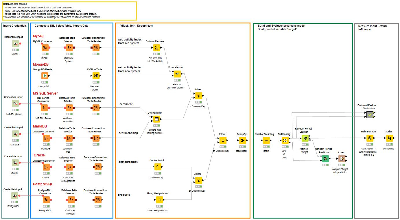
Train a Predictive Model
Most of our six datasets contain information about all of the customers. Only the web activity datasets alone do not cover all customers. However, together they do. The old web activity dataset is concatenated with the new web activity dataset. After that, all data coming from all of the different data sources are adjusted, renamed, converted, and joined so that one row represents one customer, where the customer is identified by its unique customer key.
Note. Notice the usage of a GroupBy node to perform a deduplication operation. Indeed, grouping data rows on all features allows for removal of identical rows.
The resulting dataset is then partitioned and used to train a machine learning model. As machine learning model, we chose a random forest with 100 trees and we trained it to predict the value in “Target” column. “Target” is a binary feature representing whether a customer bought a second product. So training the model to predict the value in “Target” means that we are training the model to produce the likelihood of a customer to buy a second product, given all that we already know about her/him.
The model is then applied to the test set and its performance evaluated with a Scorer node. The model accuracy was calculated to be around 77%.
Measuring the Influence of Input Features
A very frequent task in data analytics projects is to determine the influence of the input features on the trained model. There are many solutions to that, which also depend on the kind of predictive model that has been adopted.
A classic solution that works with all predictive algorithms is the backward feature elimination procedure (or its analogous forward feature construction).
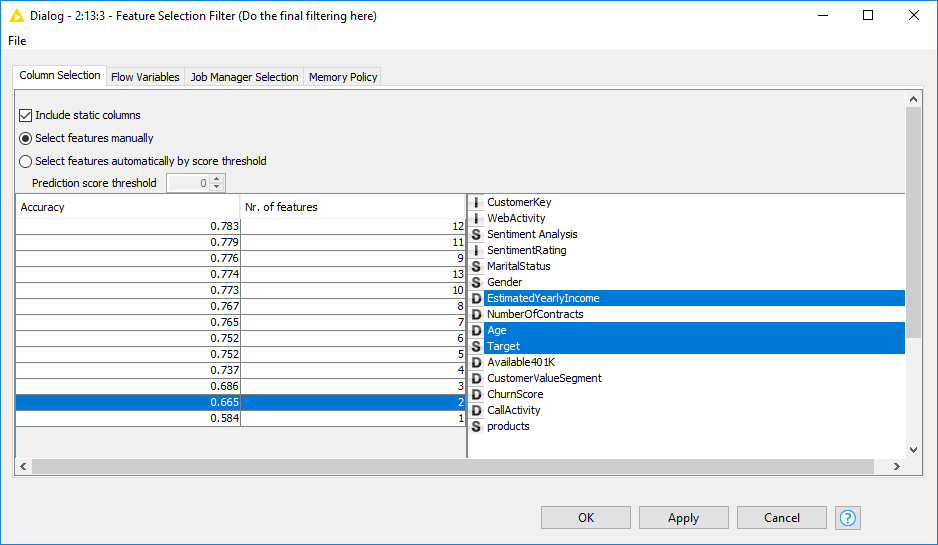
Backward Feature Elimination starts with all N input features and progressively removes one to see how this affects the model performance. The input feature whose removal lowers the model’s performance the least is left out. This step is repeated until the model’s performance is worsened considerably. The subset of input features producing a high accuracy (or a low error) represents the subset of most influential input features. Of course, the definition of high accuracy (or low error) is arbitrary. It could mean the highest accuracy or a high enough accuracy for our purposes.
The metanode, named “Backward Feature Elimination” and available in the Node Repository under KNIME Labs/Wide Data/Feature Selection, implements exactly this procedure. The final node in the loop, named “Feature Selection Filter”, produces a summary of the model performance, for all steps where the input feature with lowest influence had been removed.
Remember that the Backward Feature Elimination procedure becomes slower with the higher number of input features. It works well with a limited number of input features, but avoid using it to investigate hundreds of them.
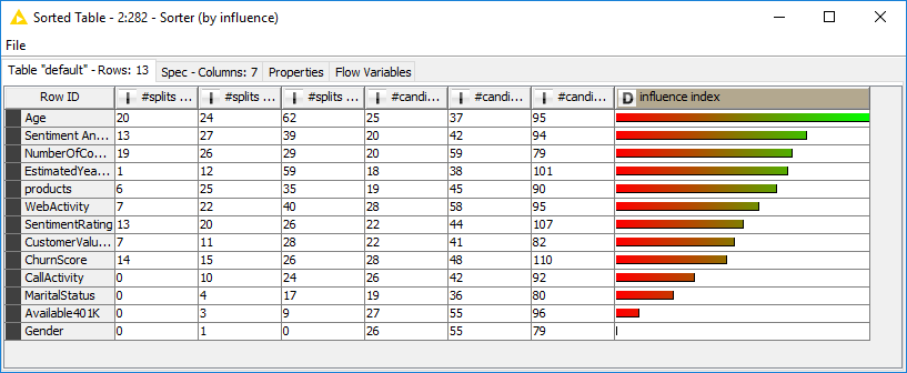
In addition, a random forest offers a higher degree of interpretability with respect to other machine learning models. One of the output ports of the Random Forest Learner node provides the number of times an input feature has been the candidate for a split and the number of times it has actually been chosen for the split, for levels 0, 1, and 2 across all trees in the forest. For each input feature, we subsequently defined a heuristic measure of influence, borrowed from the KNIME whitepaper “Seven Techniques for Data Dimensionality Reduction”, as:
The input features with highest influence indices are the most influential ones on the model performance.

The final workflow is shown in figure 3 and it is downloadable from the KNIME EXAMPLES server under: 01_Data_Access/02_Databases/08_Database_Jam_Session01_Data_Access/02_Databases/08_Database_Jam_Session*.
In figure 3 you can see the five parts of our workflow: Credentials Definition, Database Connections and Data Retrieval, Data Blending to reach one single data table, Predictive Model Training, and Influence Measure of Input Features.
The Results
Yes, data from all of these databases do blend!
In this experiment, we blended data from six, SQL based and noSQL, databases - Oracle, MongoDB, MySQL, MariaDB, SQL Server, and PostgreSQL – to reach one single data table summarizing all available information about our customers.
In this same experiment, we also trained a random forest model to predict the likelihood of a customer buying a second product.
Finally, we measured each input feature’s influence on the final predictions, using a Backward Feature Elimination procedure and a heuristic influence measure based on the numbers of splits and candidates in the random forest. Results from both procedures are shown in figures 4 and 5. Both figures show the prominent role of Age and Estimated Yearly Income and the negligible role of Gender, when predicting whether customer will buy a second product.
This whole predictive and influence analysis was made possible purely because of the data blending operation involving the many different database sources. The main result is therefore another yes! Data can be retrieved from different databases and they all blend!
The data and use case for this post are from the basic and advanced course on KNIME Analytics Platform. The course, naturally, covers much more and goes into far more detail than what we have had the chance to show here.
Note. Just in case, you got intrigued and you want to know more about the courses that KNIME offers, you can refer to the course web page on the KNIME web site. Here you can find the courses schedule and a description of their content. In particular, the slides for the basic and advanced course can now be downloaded for free from https://www.knime.org/course-materials-download-registration-page.
Coming Next …
If you enjoyed this, please share it generously and let us know your ideas for future blends.