The recent explosion of data set size, in number of records and attributes, has triggered the development of a number of big data platforms as well as parallel data analytics algorithms. At the same time though, it has pushed for usage of data dimensionality reduction procedures. Indeed, more is not always better. Large amounts of data might sometimes produce worse performances in data analytics applications.
One of my most recent projects happened to be about churn prediction and to use the 2009 KDD Challenge large data set. The particularity of this data set consists of its very high dimensionality with 15K data columns. Most data mining algorithms are column-wise implemented, which makes them slower and slower on a growing number of data columns. The first milestone of the project was then to reduce the number of columns in the data set and lose the smallest amount of information possible at the same time.
Using the project as an excuse, we started exploring the state-of-the-art on dimensionality reduction techniques currently available and accepted in the data analytics landscape.
- Missing Values Ratio. Data columns with too many missing values are unlikely to carry much useful information. Thus data columns with number of missing values greater than a given threshold can be removed. The higher the threshold, the more aggressive the reduction.
- Low Variance Filter. Similarly to the previous technique, data columns with little changes in the data carry little information. Thus all data columns with variance lower than a given threshold are removed. A word of caution: variance is range dependent; therefore normalization is required before applying this technique.
- High Correlation Filter. Data columns with very similar trends are also likely to carry very similar information. In this case, only one of them will suffice to feed the machine learning model. Here we calculate the correlation coefficient between numerical columns and between nominal columns as the Pearson’s Product Moment Coefficient and the Pearson's chi square value respectively. Pairs of columns with correlation coefficient higher than a threshold are reduced to only one. A word of caution: correlation is scale sensitive; therefore column normalization is required for a meaningful correlation comparison.
- Random Forests / Ensemble Trees. Decision Tree Ensembles, also referred to as random forests, are useful for feature selection in addition to being effective classifiers. One approach to dimensionality reduction is to generate a large and carefully constructed set of trees against a target attribute and then use each attribute’s usage statistics to find the most informative subset of features. Specifically, we can generate a large set (2000) of very shallow trees (2 levels), with each tree being trained on a small fraction (3) of the total number of attributes. If an attribute is often selected as best split, it is most likely an informative feature to retain. A score calculated on the attribute usage statistics in the random forest tells us ‒ relative to the other attributes ‒ which are the most predictive attributes.
- Principal Component Analysis (PCA). Principal Component Analysis (PCA) is a statistical procedure that orthogonally transforms the original n coordinates of a data set into a new set of n coordinates called principal components. As a result of the transformation, the first principal component has the largest possible variance; each succeeding component has the highest possible variance under the constraint that it is orthogonal to (i.e., uncorrelated with) the preceding components. Keeping only the first m < n components reduces the data dimensionality while retaining most of the data information, i.e. the variation in the data. Notice that the PCA transformation is sensitive to the relative scaling of the original variables. Data column ranges need to be normalized before applying PCA. Also notice that the new coordinates (PCs) are not real system-produced variables anymore. Applying PCA to your data set loses its interpretability. If interpretability of the results is important for your analysis, PCA is not the transformation for your project.
- Backward Feature Elimination. In this technique, at a given iteration, the selected classification algorithm is trained on n input features. Then we remove one input feature at a time and train the same model on n-1 input features n times. The input feature whose removal has produced the smallest increase in the error rate is removed, leaving us with n-1 input features. The classification is then repeated using n-2 features, and so on. Each iteration k produces a model trained on n-k features and an error rate e(k). Selecting the maximum tolerable error rate, we define the smallest number of features necessary to reach that classification performance with the selected machine learning algorithm.
- Forward Feature Construction. This is the inverse process to the Backward Feature Elimination. We start with 1 feature only, progressively adding 1 feature at a time, i.e. the feature that produces the highest increase in performance. Both algorithms, Backward Feature Elimination and Forward Feature Construction, are quite time and computationally expensive. They are practically only applicable to a data set with an already relatively low number of input columns.
We picked this chance to compare those techniques on the smaller data set of the 2009 KDD challenge in terms of reduction ratio, degrading accuracy, and speed. The final accuracy and its degradation depend, of course, on the model selected for the analysis. Thus, the compromise between reduction ratio and final accuracy is optimized against a bag of three specific models: decision tree, neural networks, and naïve Bayes.
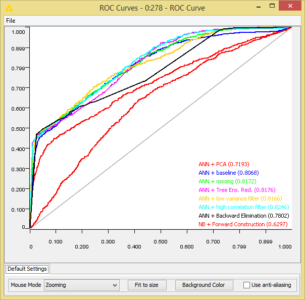
Running the optimization loop, the best cutoffs, in terms of lowest number of columns and best accuracy, were determined for each one of the seven dimensionality reduction techniques and for the best performing model. The final best model performance, as accuracy and Area under the ROC Curve, was compared with the performance of the baseline algorithm using all input features. Results of this comparison are reported in the table below.
Notice that the highest reduction ratio without performance degradation is obtained by analyzing the decision cuts in many random forests (Random Forests/Ensemble Trees). However, even just counting the number of missing values, measuring the column variance, and measuring the correlation of pairs of columns can lead to a satisfactory reduction rate while keeping performance unaltered with respect to the baseline models.
What we have learned from this little review exercise, is that dimensionality reduction is not only useful to speed up algorithm execution, but also to improve model performance. The Area under the Curve (AuC) in the table shows a slight increase on the test data, when the missing value ratio, the low variance filter, the high correlation filter criteria, or the random forests are applied.
Indeed, in the era of big data, when more is axiomatically better, we have re-discovered that too many noisy or even faulty input data columns often lead to a less than desirable algorithm performance. Removing un-informative or even worse dis-informative input attributes might help build a model on more extensive data regions, with more general classification rules, and overall with better performances on new unseen data.
Recently, we asked data analysts on a LinkedIn group for the most used dimensionality reduction techniques, besides the seven described in this blog post. The answers involved Random Projections, NMF, (Stacked) Auto-encoders, Chi-square or Information Gain, Multidimensional Scaling, Correspondence Analysis, Factor Analysis, Clustering, and Bayesian Models. Thanks to Asterios Stergioudis, Raoul Savos, and Michael Will who provided the suggestions on the LinkedIn group.
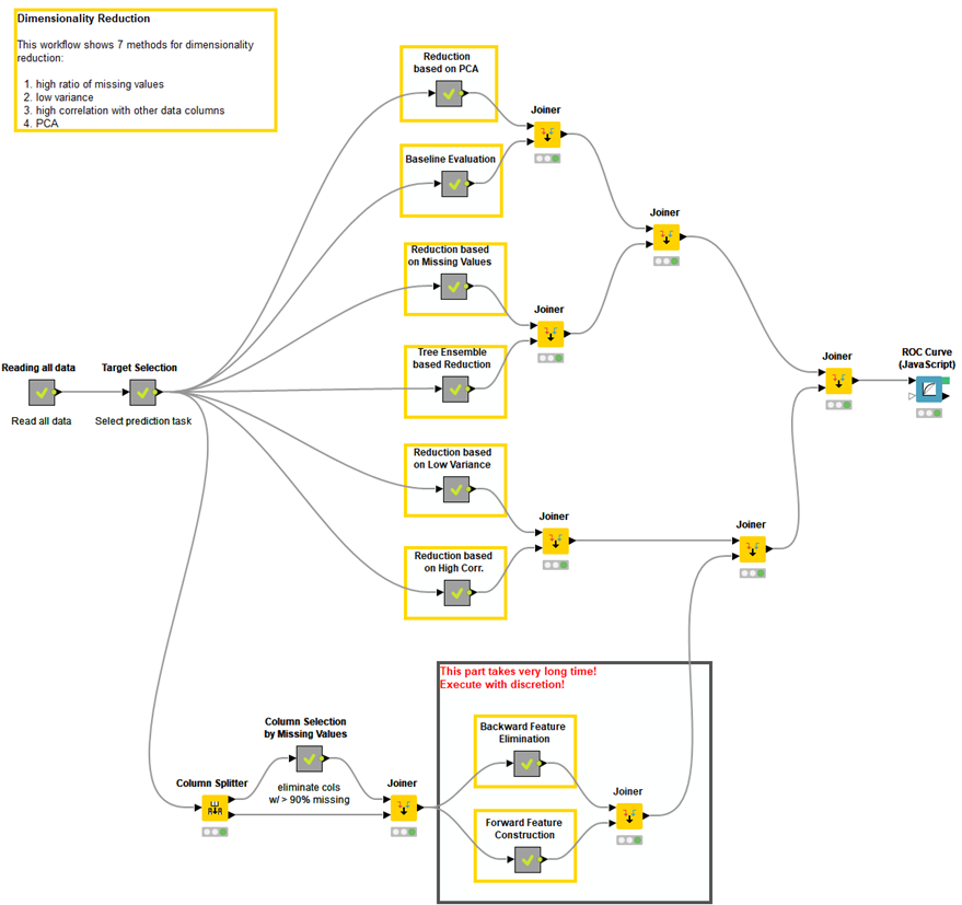
The workflows described in this blog post are available here on the KNIME Hub.
Both small and large data sets from the 2009 KDD Challenge can be downloaded from http://kdd.org/kdd-cup/view/kdd-cup-2009/Data.
This is just a brief summary of the whole project. If you are interested in all the tiny details, you can always read the related whitepaper, in the Whitepapers section on the KNIME web site:https://www.knime.org/files/knime_seventechniquesdatadimreduction.pdf
Below are the ROC curves for all the evaluated dimensionality reduction techniques and the best performing machine learning algorithm. The value of the area under the curve is shown in the legend.