
A probability distribution can be continuous or discrete. Discrete probability distributions count occurrences that are countable or finite and model the probabilities of random variables that have discrete values or outcomes. From modeling the number of sales or customers a company has to sports analysis – calculating the number of home runs in baseball or the number of sixes in cricket – discrete probability distributions will be of great use.
In this blog post, we will focus on discrete probability distributions and build a KNIME workflow to visualize 4 different discrete distributions of our data. In order to help understand the importance of discrete probability distributions we will:
- Provide a theoretical background of 4 common discrete probability distributions
- Provide a graphical understanding of them
- Build a workflow to preprocess raw data to model their discrete probability using KNIME
Download the Discrete_Distribution workflow for free from the KNIME Community Hub.
Discrete Probability Distributions in a Nutshell
A discrete probability distribution is one in which a discrete random variable X can take on a countable number of distinct values such as 0,1,2,3 and so on ‒ which can be finite, and therefore countable. For example, the number of students in the classroom or the number of traffic accidents. Since in these two examples, the random variable can take only a finite number of distinct values, it is considered a discrete random variable.
Because there are only finite values that X could assume, discrete probability distributions are expressed with a formula ‒ a Probability mass function (PMF) ‒ describing probable values and the probability associated with the random variable.
Furthermore, it’s worth stressing that in discrete probability distributions, the probability of X takes on only one specific value. Suppose, for example, that we have a discrete probability distribution for modeling the number of trades an investor makes in a day. What is the probability that an investor will have a trade of exactly 0 or 1 or 2 times? It’s only possible to exactly measure the variable that is on a discrete scale, in other words, discrete probability distribution determines the probability of one exact measurement occurring.
4 Common Types of Discrete Probability Distributions
In this section, we will go over the theoretical definition and graphical visualization of 4 common discrete probability distributions (i.e., Geometric, Binomial, Negative Binomial, and Poisson), look at examples and discuss why each distribution is important.
Before we dive into different distributions, let’s understand the meaning of a Bernoulli trial ‒ a concept that is especially relevant for the first 3 distributions. A Bernoulli trial is an experiment that can only have two outcomes, success and failure. This can also be framed as a yes or no question. For instance, football fans might have asked whether the FIFA World Cup 2022 would take place in Qatar? Or imagine yourself standing at the altar, are you going to say yes or no to the person standing in front of you? In a more general sense, in any event, a Bernoulli trial can be defined as whether the event occurred or not.
1. Geometric Distribution
Geometric distribution is a type of discrete probability distribution that describes the probability of the number of successive failures before a success is obtained in a Bernoulli trial. Notice that this distribution can have an indefinite number of trials until the first success is obtained. Only then does the Bernouli trial stop. The geometric distribution has one parameter, p, which is the probability of success for each trial. Businesses often use the geometric distribution to do a cost-benefit analysis to estimate the financial benefits of making a certain decision, or to estimate in advance an approximate number of customers that may give a positive product feedback after a number of negative feedbacks.
In geometric distributions, there are three important assumptions:
- The trials are independent of each other.
- For each trial, there are only two possible outcomes (success or failure).
- The probability of success, p, remains the same on every trial.
The graph of the geometric distribution with different probabilities of success is displayed below.
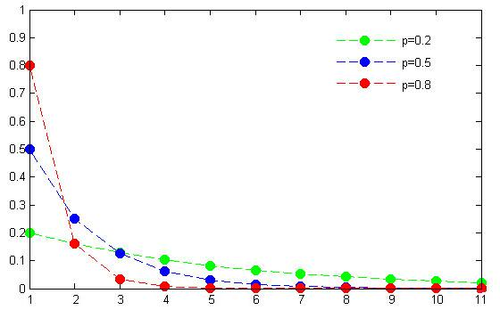
The formula of the PMF to calculate the probability of success in the kth trial of a geometric distribution is given below:
P(X = k) = (1 - p)k - 1p
where k = 1, 2, 3, 4, ...., each with the probability of success p; and (1 – p) is the probability of failure. The above formula is used for modeling the number of trials up to and including the first success.
It is noteworthy to mention that the geometric distribution is the discrete cousin of the exponential distribution. Just like in the exponential distribution which is used to model the time elapsed before a given event occurs, if Bernoulli experiments are performed at equal time intervals, the geometric distribution then models time (discrete units) before we obtain the first success. Another important property that is common is the memoryless property. Just like in the exponential distribution, geometric distributions are independent of previous trials.
2. Binomial Distribution
Binomial distribution is a type of discrete probability distribution that is used to represent the number of successes in a sequence of specified trials – each having only two possible results: success or failure. The binomial distribution requires two parameters: p, the probability of success for each trial; and n, the number of trials. When n = 1, the binomial distribution is called a Bernoulli distribution. The binomial distribution is prominently used in the field of drugs and medicine. For example, whenever a new drug is invented, its effectiveness can be represented by two outcomes, i.e., whether the drug cures the disease or it does not. Likewise, banks use the binomial distribution to estimate the chances that a particular credit card transaction is fraudulent or not.
In the binomial distributions, there are four important assumptions:
- The number of trials n is fixed.
- Each trial is independent.
- Each trial has just two possible outcomes (success or failure).
-
The probability of success, p, is the same on every trial.
The graph of the binomial distribution with different values of p and n is displayed below.
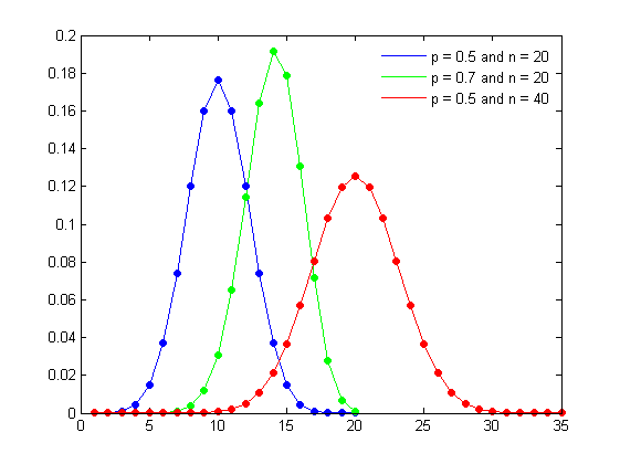
When p = 0.5, the distribution is symmetric around the mean, regardless of the value of n. When p > 0.5, the distribution is skewed to the left. When p p is to 0.5 and the larger the number of observations in the sample, the more symmetrical the distribution will be. In this case a reasonable approximation to the binomial distribution is given by the normal distribution.
The formula of the PMF to calculate binomial distribution is given below:
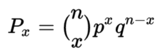
where x is the number of successes desired within n fixed trials,
is the number of combinations, p is the probability of success in a single trial, and q is the probability of failure in a single trial (1 – p).
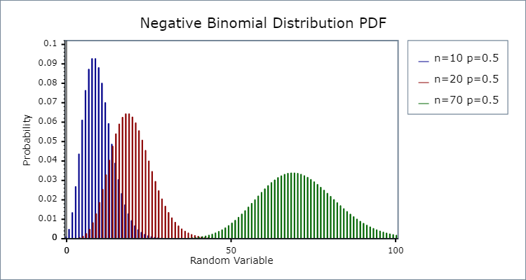
3. Negative Binomial Distribution
Negative Binomial Distribution is a discrete probability distribution that models the number of failures in a sequence of independent and identically distributed Bernoulli trials before a specified number of successes occurs. The negative binomial distribution has three parameters: r, the number of successes; n, the number of trials; and p, the probability of success for each trial. For example, consider studies of disease transmission, where the number of infections caused by a certain disease may indicate an epidemic, or the number of job interviews one must go on before receiving multiple job offers; these events could be modeled by a negative binomial distribution.
In negative binomial distributions, there are three important assumptions:
- Each trial is independent.
- For each trial, there are only two possible outcomes (success or failure).
- The probability of success, p, is the same for each trial.
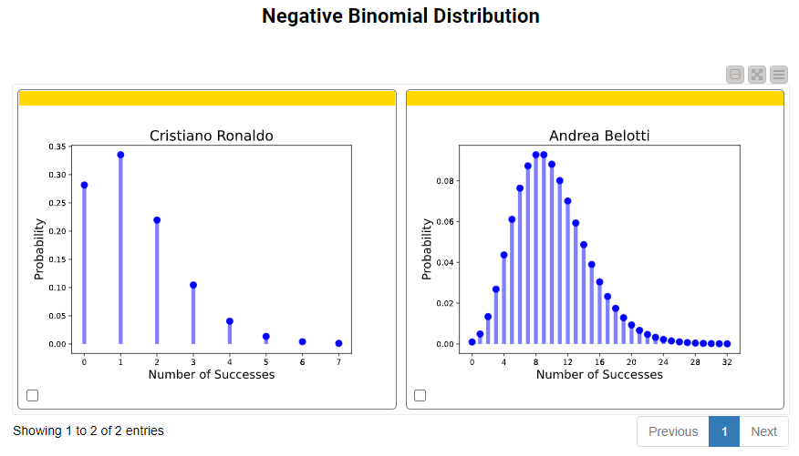
The graph of the negative binomial distribution with different values of p and n is displayed below.
The formula of the PMF to calculate Negative Binomial distribution is given below:
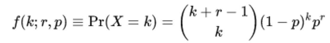
Where
is the binomial coefficient, r > 0 is the number of successes, k is the number of failures (n – r), and p is the probability of success on each trial.
One interesting characteristic of the negative binomial distribution that is worth noticing is that if r = 1 then the distribution tends to be a geometric distribution with parameter p.
4. Poisson Distribution
Poisson distributions describe the probability of an event happening a certain number of times k within a fixed interval of time. This distribution has only one parameter, λ which is the expected rate of occurrences (mean number) of events. An intuitive way of looking at Poisson distribution is that there is a small chance that an event will occur on any one trial in which there is a large number of opportunities for the event to occur. This is why this distribution is often used to describe rare events. For example, the number of cases of bankruptcies filed every month, storms in your neighboring city, and even the number of people visiting a local bakery, all follow the Poisson distribution.
In Poisson distributions, there are two important assumptions:
- The occurrences of events are independent of each other.
- The expected rate of occurrences, λ, in a fixed interval is known.
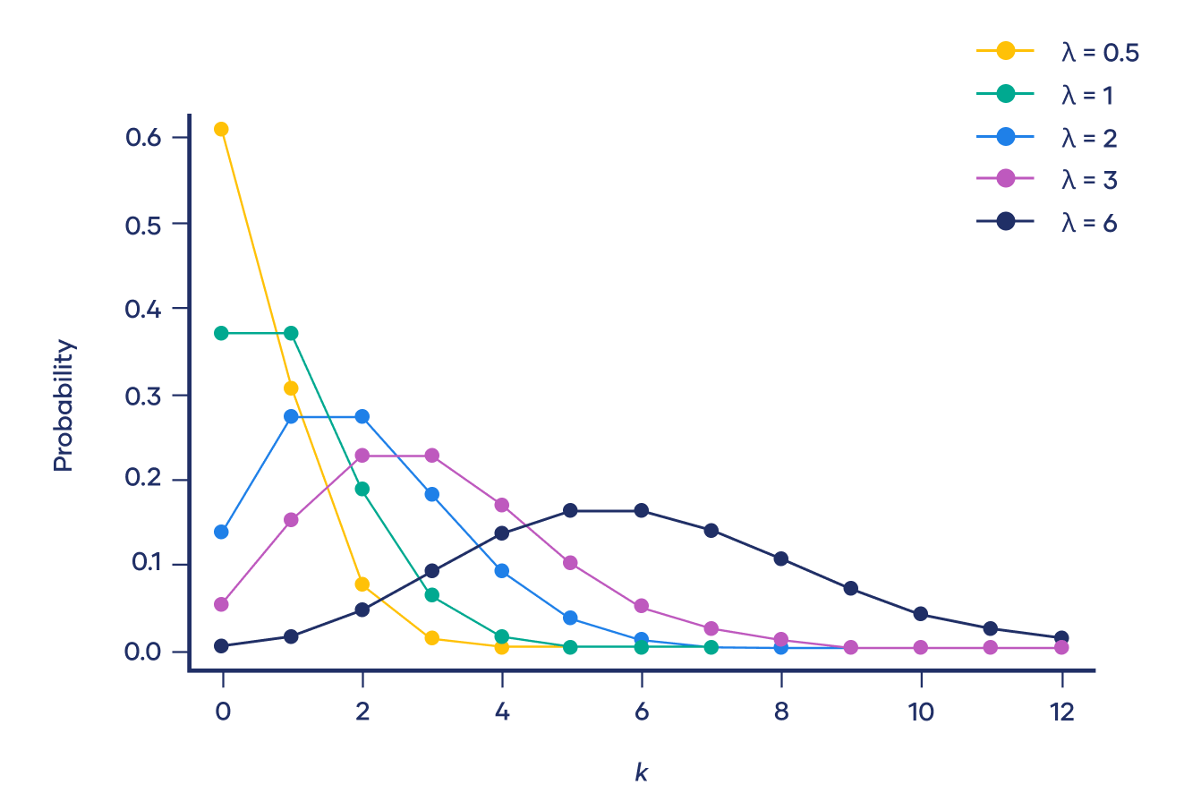
The graph of the Poisson distribution with different λ values is displayed below:
The formula of the PMF to calculate Poisson distribution, with parameter λ > 0 is given below:
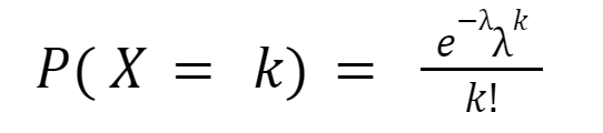
Where k is the number of occurrences (k = 0,1, 2,...), e is the Euler number and λ is the expected rate of occurrences.
The most probable number of events is represented by the peak of the distribution (Fig. 4). It is worth noting that for smaller values of λ, the distribution is strongly right-skewed but, as λ increases, the distribution looks more and more similar to a normal distribution. Indeed, when λ = 10 or greater, a normal distribution is a good approximation of the Poisson distribution.
Find Discrete Probability Distributions with KNIME
After a few theoretical insights, we are ready to build a KNIME workflow to find, understand and visualize different discrete probability distributions for our data. To do that, we relied on the KNIME Python Integration and built a configurable component for ease of reusability (Fig. 5).
Check out How to Set Up the Python Extension and the KNIME Python Integration Installation Guide to know more.
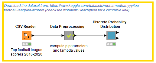
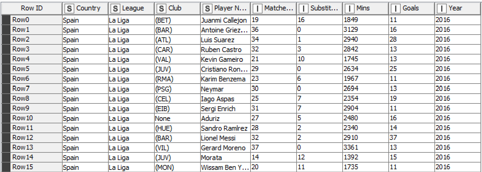
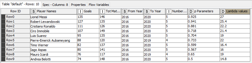
The Discrete Probability Distribution component is a Python-based component and uses the scipy.stats library in the Python Script node to find the probability values and visualize discrete distribution plots. For this example workflow, we used the Top Football Leagues Scorers (2016-2020) dataset. It contains league tables and statistics from some of the top football competitions from all around the world, including the English Premier League, English Championship, Spanish La Liga, Italian Serie A, German Bundesliga, French Ligue 1, US MLS and Brazilian Série A. Before we dive into the different uses of this component, let’s understand the Data Preprocessing metanode (Fig. 6).

The key operations in this metanode help us manipulate, clean and normalize the dataset and filter the top 10 football players by the number of goals. It also helps us calculate p parameters for each player, i.e. is the probability of a single success, and lambda values, i.e. the expected rate of occurrences (mean number) of events. Below we see how the data is transformed from its raw state (Fig. 7) to the preprocessed state needed as input for the component (Fig. 8).
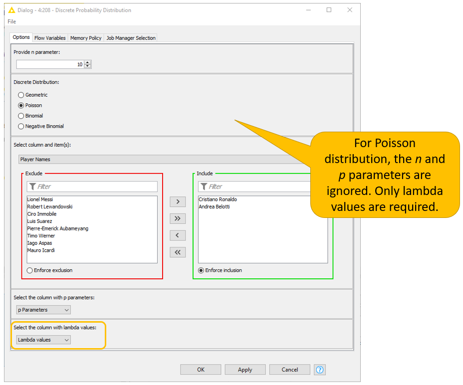
The configuration window of the Discrete Probability Distribution component (Fig. 9) allows the user to:
- Provide an n parameter representing the number of trials or the number of successes according to the distribution it refers to. For the Poisson distribution, this parameter is not required;
- Select the desired discrete probability distribution;
- Select one or multiple rows of a particular column;
- Select the columns in the dataset containing p parameters or lambda values. Notice that the p parameters are required only for the geometric, binomial and negative binomial distributions, whereas lambda values are required exclusively for the Poisson distribution. If the p parameters or lambda values are input when not required, the component automatically ignores them.
For example, we might want to inspect the Poisson probability distribution for Cristiano Ronaldo and Andrea Belotti (see Fig. 9).
The workflow wrapped inside the component relies on error handling nodes to account for error in the Python Scripts nodes, uses the Conda Environment Propagation node to install necessary Python libraries and enhance workflow portability across different OSs, and displays results with JavaScript-based visualization nodes.
Probability Values & Visualization of Distributions
Let’s find and visualize the geometric probability distribution of Cristiano Ronaldo and Andrea Belotti. In Fig. 10, we set the number of trials to 10 to observe how the probability of success in each particular trial behaves.
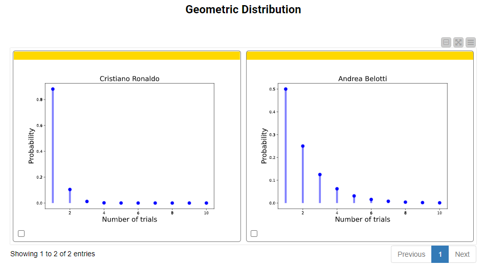
Plots show only values on the x-axis whose probabilities fall in the range between 0.00001 and 0.99999. Exception: in the Geometric Probability Distribution probability values are reported for each trial regardless of the value range.
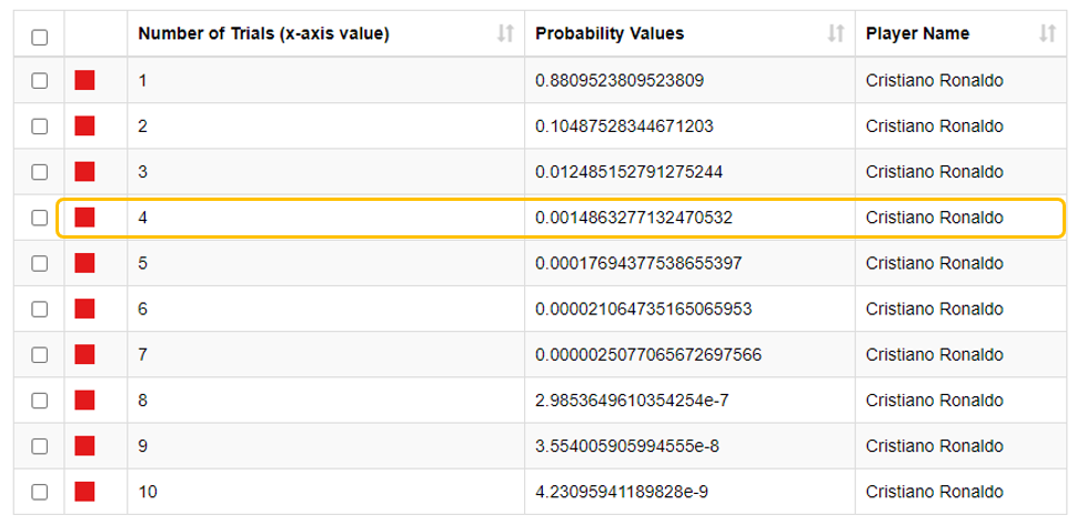
If we zoom in on Cristiano Ronaldo, we can see the table of probability values in Fig. 12. Using the computed p parameter (0.881) from the input table, we can see that if he was unsuccessful in shooting a goal in the first three independent trials, then the probability of him shooting a goal in the fourth independent trial drastically drops to 0.00148.
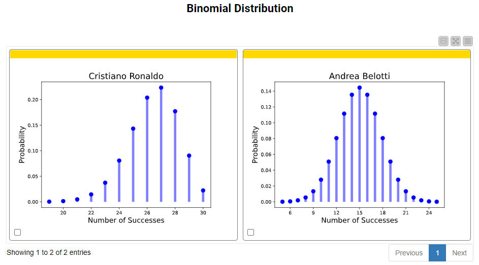
Next, it’s time to explore the binomial distribution. We set n, the number of trials, to 30 and plot the probability values in Fig. 12. It is important to note that in these and in the remaining probability distribution plots, the x-axes reflect the number of successes, and not the number of trials. Based on the input p parameters, we can see that the probability of Andrea Belotti shooting exactly 15 successful shots in 30 trials is 0.14. Similarly, the probability of Cristiano Ronaldo shooting exactly 27 successful shots in 30 trials is 0.22.
In the case of the negative binomial distribution. To obtain the plots below, we set the number of successes to 10, and rely again on the p parameters. For Andrea Bellotti, the probability of having 9 failures before the 10th success of shooting a goal is 0.0927. Similarly, for Cristiano Ronaldo, the probability of having 4 failures before the 5th success of shooting a goal is 0.04.
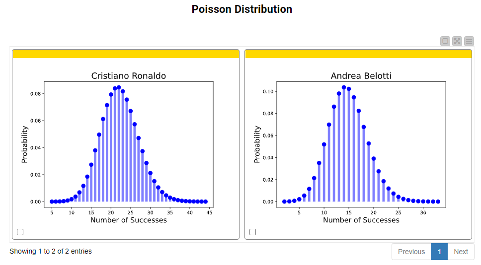
Finally, we explore the Poisson distribution for the same players. In Fig. 14, we see the Poisson distribution plot with the total number of successful shots within a set interval. The n parameter is not required in this case, since the component is designed to display all the possible number of times an event occurs.
For the Poisson distribution, we need to consider lambda as a key parameter. Since the lambda value varies for each player – i.e, the average number of successful shots of Cristiano Ronaldo is higher than that of Andrea Belotti – Cristiano Ronaldo has more successive shots within the range. It follows that the associated probability of each shot within the range also changes. Consistent with the theory, as the lambda value increases (>= 10) the Poisson distribution can be approximated by a normal distribution. Likewise, for less rare events (i.e. Ronaldo's successive shots), the peak of the distribution has a much lower probability value.
The probability values obtained for each plot are also available in a table format and can be viewed in the component interactive view.
Use the Discrete Probability Distribution Component to Know Your Data
It is very important to know and understand different discrete probability distributions in order to understand your data and conduct proper statistical analysis. The Discrete Probability Distribution component is easy to use and gives you heaps of information about the distribution and the probability values.
Use your data as input for this component, select the desired distribution you want to visualize, and input the other parameters in the configuration window. The component does the rest for you! It will provide you with the visualization of your desired discrete distribution for your data, as well as probability values. Curious? Try it out!