Three New Techniques for Data Dimensionality Reduction in Machine Learning

As first published in The New Stack.

The full big data explosion has convinced us that more is better. While it is of course true that a large amount of training data helps the machine learning model to learn more rules and better generalize to new data, it is also true that an indiscriminate addition of low-quality data and input features might introduce too much noise and, at the same time, considerably slow down the training algorithm.

So, in the presence of a dataset with a very high number of data columns, it is good practice to wonder how many of these data features are actually really informative for the model. A number of techniques for data-dimensionality reduction are available to estimate how informative each column is and, if needed, to skim it off the dataset.

Back in 2015, we began publishing a review¹ of the seven most commonly used techniques for data-dimensionality reduction, including:

• Ratio of missing values
• Low variance in the column values
• High correlation between two columns
• Principal component analysis (PCA)
• Candidates and split columns in a random forest
• Backward feature elimination
• Forward feature construction

Those are traditional techniques commonly applied to reduce the dimensionality of a dataset by removing all of the columns that either do not bring much information or no new information. Since then, we have started to use three additional techniques, also quite commonly used, and have decided to add them to the list as well.

1. Linear discriminant analysis (LDA)
2. Neural autoencoder
3. t-distributed stochastic neighbor embedding (t-SNE)

Let’s start with the three techniques recently added and then move backwards in time with a review of the seven original techniques.

In our first review of data dimensionality reduction techniques, we used the two datasets from the 2009 KDD Challenge - the large dataset and the small dataset. The particularity of the large dataset is its very high dimensionality with 15,000 data columns. Most data mining algorithms are implemented columnwise, which makes them slower and slower as the number of data columns increases. This dataset definitely brings out the slowness of a number of machine learning algorithms.

The 2009 KDD Challenge small dataset is definitely lower dimensional than the large dataset but is still characterized by a considerable number of columns: 230 input features and three possible target features. The number of data rows is the same as in the large dataset: 50,000. In this review, for computational reasons, we will focus on the small dataset to show just how effective the proposed techniques are in reducing dimensionality. The dataset is big enough to prove the point in data-dimensionality reduction and small enough to do so in a reasonable amount of time.

Let’s proceed now with the (re)implementation and comparison of 10 state-of-the-art dimensionality reduction techniques, all currently available and commonly used in the data analytics landscape.

Let’s start with the three newly added techniques:

1. Linear Discriminant Analysis (LDA)
2. Neural autoencoder
3. t-distributed Stochastic Neighbor Embedding (t-SNE)

A number m of linear combinations (discriminant functions) of the n input features, with m < n, are produced to be uncorrelated and to maximize class separation. These discriminant functions become the new basis for the dataset. All numeric columns in the dataset are projected onto these linear discriminant functions, effectively moving the dataset from the n-dimensionality to the m-dimensionality.

In order to apply the LDA technique for dimensionality reduction, the target column has to be selected first. The maximum number of reduced dimensions m is the number of classes in the target column minus one, or if smaller, the number of numeric columns in the data. Notice that linear discriminant analysis assumes that the target classes follow a multivariate normal distribution with the same variance but with a different mean for each class.²

An autoencoder is a neural network, with as many n output units as input units, at least one hidden layer with m units where m < n, and trained with the backpropagation algorithm to reproduce the input vector onto the output layer. It reduces the numeric columns in the data by using the output of the hidden layer to represent the input vector.

The first part of the autoencoder — from the input layer to the hidden layer of m units — is called the encoder. It compresses the n dimensions of the input dataset into an m-dimensional space. The second part of the autoencoder — from the hidden layer to the output layer — is known as the decoder. The decoder expands the data vector from an m-dimensional space into the original n-dimensional dataset and brings the data back to their original values.³

This technique reduces the n numeric columns in the dataset to fewer dimensions m (m < n) based on nonlinear local relationships among the data points. Specifically, it models each high-dimensional object by a two- or three-dimensional point in such a way that similar objects are modeled by nearby points and dissimilar objects are modeled by distant points in the new lower dimensional space.

In the first step, the data points are modeled through a multivariate normal distribution of the numeric columns. In the second step, this distribution is replaced by a lower dimensional t-distribution, which follows the original multivariate normal distribution as closely as possible. The t-distribution gives the probability of picking another point in the dataset as a neighbor to the current point in the lower dimensional space. The perplexity parameter controls the density of the data as the “effective number of neighbors for any point.” The greater the value of the perplexity, the more global structure is considered in the data. The t-SNE technique works only on the current dataset. It is not possible to export the model to apply it to new data.⁴

Here is a brief review of our original seven techniques for dimensionality reduction:

• Missing Values Ratio. Data columns with too many missing values are unlikely to carry much useful information. Thus, data columns with a ratio of missing values greater than a given threshold can be removed. The higher the threshold, the more aggressive the reduction.

• Low Variance Filter. Similar to the previous technique, data columns with little changes in the data carry little information. Thus, all data columns with a variance lower than a given threshold can be removed. Notice that the variance depends on the column range, and therefore normalization is required before applying this technique.

• High Correlation Filter. Data columns with very similar trends are also likely to carry very similar information, and only one of them will suffice for classification. Here we calculate the Pearson product-moment correlation coefficient between numeric columns and the Pearson’s chi-square value between nominal columns. For the final classification, we only retain one column of each pair of columns whose pairwise correlation exceeds a given threshold. Notice that correlation depends on the column range, and therefore, normalization is required before applying this technique.

• Random Forests/Ensemble Trees. Decision tree ensembles, often called random forests, are useful for column selection in addition to being effective classifiers. Here we generate a large and carefully constructed set of trees to predict the target classes and then use each column’s usage statistics to find the most informative subset of columns. We generate a large set (2,000) of very shallow trees (two levels), and each tree is trained on a small fraction (three columns) of the total number of columns. If a column is often selected as the best split, it is very likely to be an informative column that we should keep. For all columns, we calculate a score as the number of times that the column was selected for the split, divided by the number of times in which it was a candidate. The most predictive columns are those with the highest scores.

• Principal Component Analysis (PCA). Principal component analysis (PCA) is a statistical procedure that orthogonally transforms the original n numeric dimensions of a dataset into a new set of n dimensions called principal components. As a result of the transformation, the first principal component has the largest possible variance; each succeeding principal component has the highest possible variance under the constraint that it is orthogonal to (i.e., uncorrelated with) the preceding principal components. Keeping only the first m < n principal components reduces the data dimensionality while retaining most of the data information, i.e., variation in the data. Notice that the PCA transformation is sensitive to the relative scaling of the original columns, and therefore, the data need to be normalized before applying PCA. Also notice that the new coordinates (PCs) are not real, system-produced variables anymore. Applying PCA to your dataset loses its interpretability. If interpretability of the results is important for your analysis, PCA is not the transformation that you should apply.

• Backward Feature Elimination. In this technique, at a given iteration, the selected classification algorithm is trained on n input columns. Then we remove one input column at a time and train the same model on n-1 columns. The input column whose removal has produced the smallest increase in the error rate is removed, leaving us with n-1 input columns. The classification is then repeated using n-2 columns, and so on. Each iteration k produces a model trained on n-k columns and an error rate e(k). By selecting the maximum tolerable error rate, we define the smallest number of columns necessary to reach that classification performance with the selected machine learning algorithm.

• Forward Feature Construction. This is the inverse process to backward feature elimination. We start with one column only, progressively adding one column at a time, i.e., the column that produces the highest increase in performance. Both algorithms, backward feature elimination and forward feature construction, are quite expensive in terms of time and computation. They are practical only when applied to a dataset with an already relatively low number of input columns.

We implemented all 10 described techniques for dimensionality reduction, applying them to the small dataset of the 2009 KDD Cup corpus. Finally, we compared them in terms of reduction ratio and classification accuracy. For dimensionality reduction techniques that are based on a threshold, the optimal threshold was selected by an optimization loop.

For some techniques, final accuracy and degradation depend on the selected classification model. Therefore, the classification model is chosen from a bag of three basic models as the best-performing model:

• Multilayer feedforward neural networks
• Naive Bayes
• Decision tree

For such techniques, the final accuracy is obtained by applying all three classification models to the reduced dataset and adopting the one that performs best.

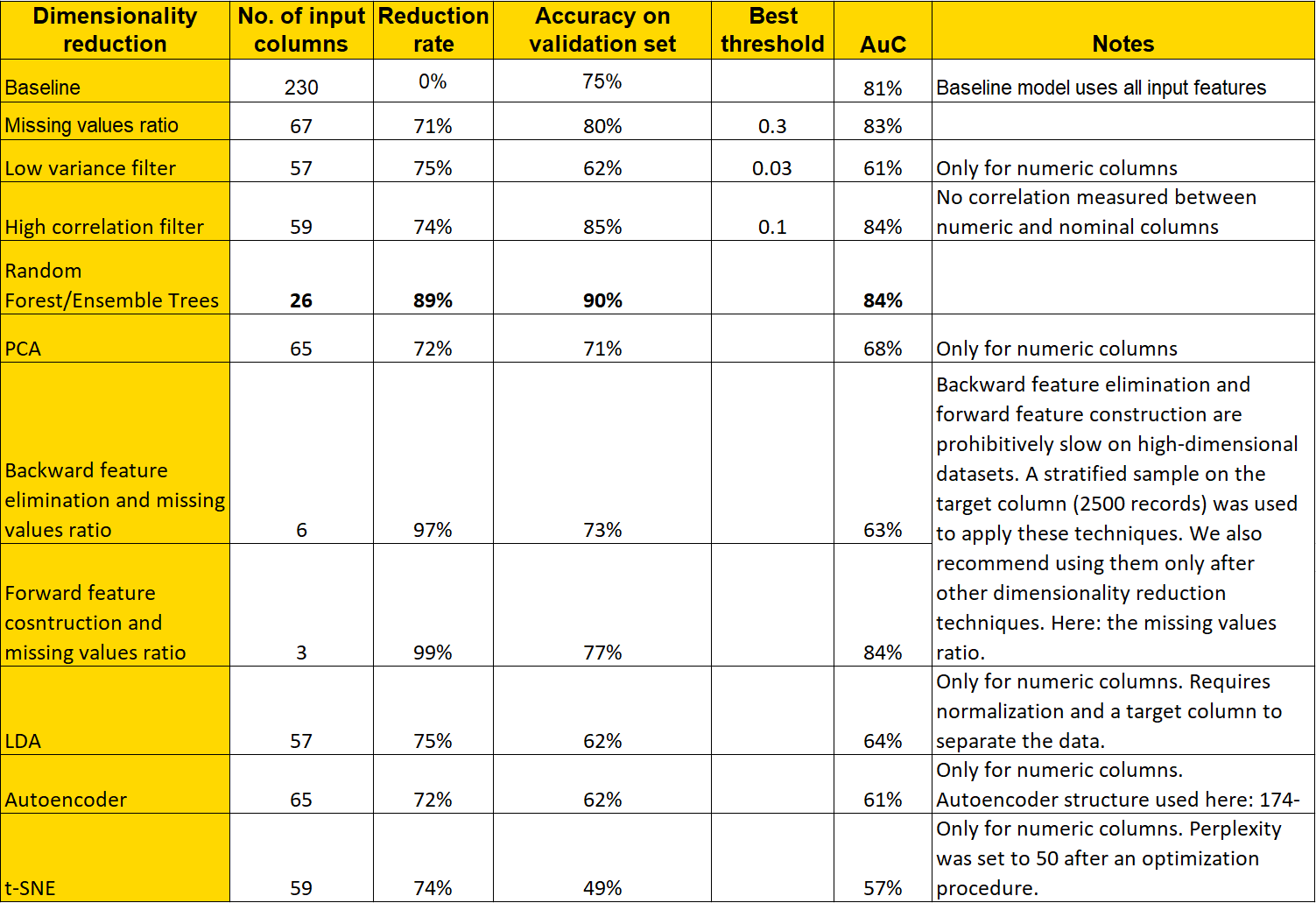
Overall accuracy and area under the curve (AUC) statistics are reported for all techniques in Table 1. We compare these statistics with the performance of the baseline algorithm that uses all columns for classification.

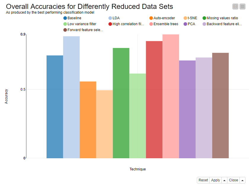
A graphical comparison of the accuracy of each reduction technique is shown in Figure 1 below. Here all reduction techniques are reported on the x-axis and the corresponding classification accuracy on the y-axis, as obtained from the best-performing model of the three basic models proposed above.

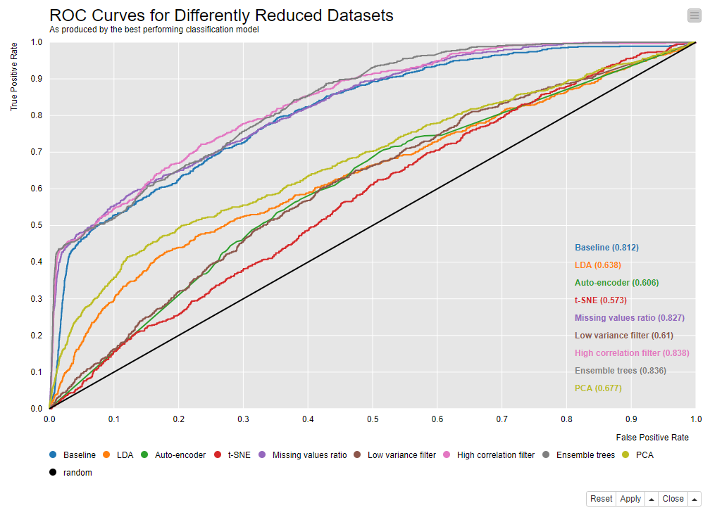
The receiver operating characteristic (ROC) curves in Figure 2 show a group of best-performing techniques: missing value ratio, high correlation filter and the ensemble tree methods.

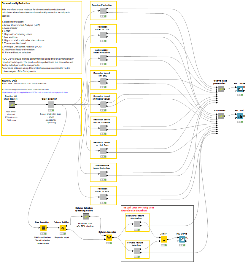
The workflow that implements and compares the 10 dimensionality reduction techniques described in this review is shown in Figure 3. In the workflow, we see 10 parallel branches plus one at the top. Each one of the 10 parallel lower branches implements one of the described techniques for data-dimensionality reduction. The first branch, however, trains the bag of classification models on the whole original dataset with 230 input features.

Each workflow branch produces the overall accuracy and the probabilities for the positive class by the best-performing classification model trained on the reduced dataset. Finally, the positive class probabilities and actual target class values are used to build the ROC curves, and a bar chart visualizes the accuracies produced by the best-performing classification model for each dataset.

You can inspect and download the workflow from the KNIME Hub.

In this article we have presented a review of ten popular techniques for data dimensionality reduction. We have actually expanded a previous existing article describing seven of them (ratio of missing values, low variance in the values of a column, high correlation between two columns, principal component analysis (PCA), candidates and split columns in a random forest, backward feature elimination, forward feature construction)

We trained a few basic machine learning models on the reduced datasets and compared the best-performing ones with each other via reduction rate, accuracy and area under the curve.

Notice that dimensionality reduction is not only useful to speed up algorithm execution but also to improve model performance.

In terms of overall accuracy and reduction rate the random, the Random Forest based technique proved to be the most effective in removing uninteresting columns and retaining most of the information for the classification task at hand. Of course, the evaluation, reduction and consequent ranking of the ten described techniques are applied here to a classification problem; we cannot generalize to effective dimensionality reduction for numerical prediction or even visualization.

Some of the techniques used in this article are complex and computationally expensive. However, as the results show, even just counting the number of missing values, measuring the column variance and the correlation of pairs of columns — and combining them with more sophisticated methods — can lead to a satisfactory reduction rate while keeping performance unaltered with respect to the baseline models.

Indeed, in the era of big data, when more is axiomatically better, we have rediscovered that too many noisy or even faulty input data columns often lead to unsatisfactory model performance. Removing uninformative — or even worse — misinformative input columns might help to train a machine learning model on more general data regions, with more general classification rules, and overall with better performances on new, unseen data.

^1. Silipo, R. (December 5, 2015). Seven Techniques for Data Dimensionality Reduction [Blog post]. Retrieved from: https://www.knime.com/blog/seven-techniques-for-data-dimensionality-reduction

^2. Linear discriminant analysis. (2019, July 19). In Wikipedia: The Free Encyclopedia. Retrieved, July 19, 2019, from https://en.wikipedia.org/wiki/Linear_discriminant_analysis

^3. Hugo Larochelle. (2013, November 15). Neural networks [6.1] : Autoencoder - definition [Video file]. Retrieved from https://youtu.be/FzS3tMl4Nsc

^4. Kurita, K. (September 14, 2018). Paper Dissected: “Visualizing Data using t-SNE” Explained [Blog post]. Retrieved from: https://mlexplained.com/2018/09/14/paper-dissected-visualizing-data-using-t-sne-explained/