Predict Blood Glucose with an LSTM on CGM Data

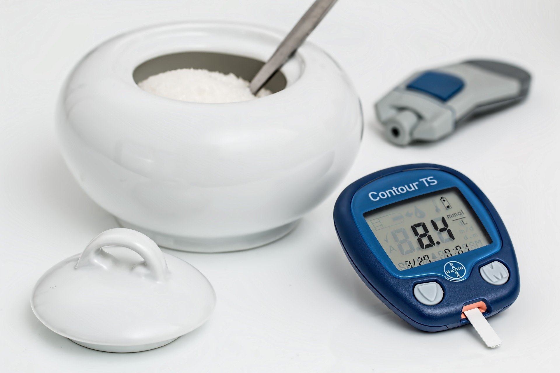
The number of people suffering from diabetes is increasing drastically worldwide. Devices called continuous glucose monitors (CGMs) exist to help make the everyday lives of diabetics easier. These tiny sensor wires are inserted under the skin, and then record blood sugar (glucose) levels at certain time intervals, transmitting the data to an app or software. This way, a user can see their current and past blood glucose levels. But wouldn’t it be great to know your future levels as well?

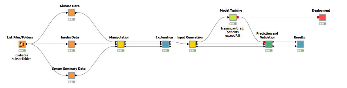
To that end, I trained an LSTM network with existing CGM data to predict future blood glucose levels. This makes it possible to recognize early on whether your sugar levels could rise or fall drastically, enabling rapid intervention. It’s a great way to make everyday life easier for diabetics, and I'll show you how to do it in KNIME. You can already see the complete workflow in Figure 1.

There are two types of diabetes: Type 1, in which the body does not produce enough or any insulin, and Type 2, in which the body doesn't use insulin properly¹. Type 2 is the most common form of diabetes, and some people can manage their blood sugar levels with a healthy diet and exercise. Others may need insulin to help control their blood sugar levels. For them, keeping track of their blood sugar is a crucial everyday task.

In this post, we will look at the D1NAMO dataset, which contains CGM blood glucose measurements and insulin dose data from Type 1 diabetes patients. The cool thing is that it contains data not only from CGMs, but also motion sensors. The participants were each monitored using the Zephyr BioHarness 3 wearable chest belt device, which recorded information on their hearts, respiration rates, and body acceleration.

Currently, software/apps which use CGMs to display one’s blood glucose levels can only show the past and current values. But wouldn’t it be helpful to know the future values as well? With this information, a diabetic could know if their blood sugar level will soon rise or sink. In my workflow, I used an LSTM network to make these kinds of predictions.

To explore the different features, I created an interactive view via a component which shows the different measurements, as seen in Figure 2. It shows measurements from "Diabetes_Patient_1" on October 1st, but you can also view other patients and dates. This is possible by combining several Line Plots that operate on the same data table and additional Value Selection Widgets, which allow me to filter the data directly in the view. I also used a new widget, the Refresh Button. With this, you no longer have to close your view to apply new settings.

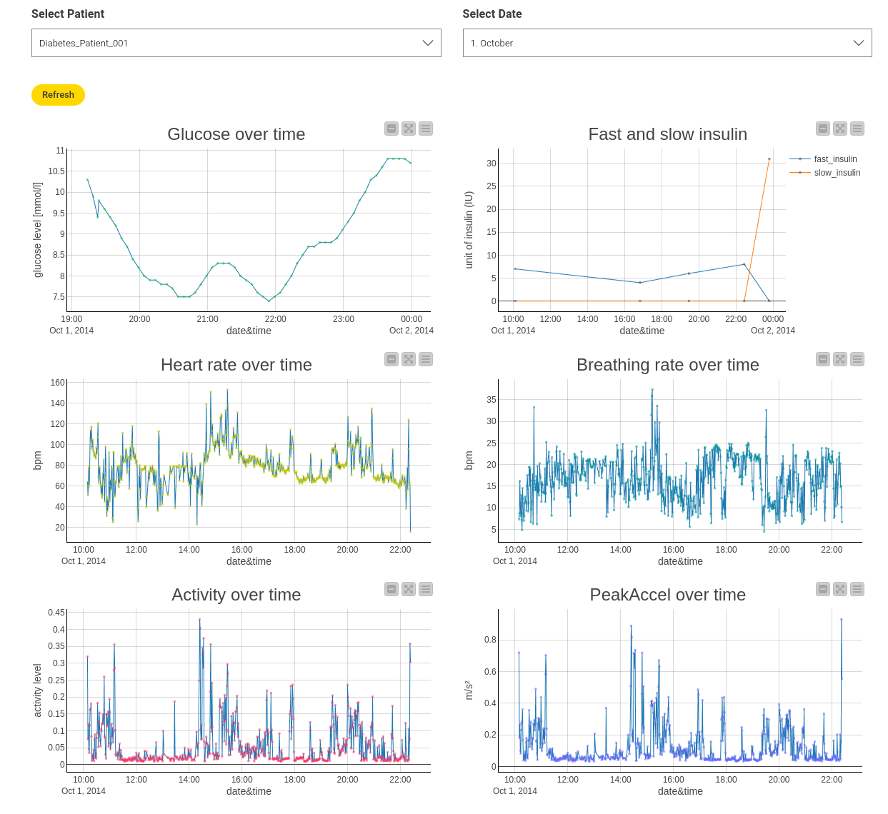
I included the features “heart rate,” “breathing rate,” “activity,” and “peak acceleration over time” in this view. “Activity” and “peak acceleration” refer to the mean and maximum acceleration magnitude measured by the sensor. Insulin values are also included, showing how much fast or slow insulin was injected at which time.

But the dataset includes more sensor data as well. If you are interested in exploring the whole set or learning more, read “The open D1NAMO dataset: A multi-modal dataset for research on non-invasive type 1 diabetes management” from Dubosson².To keep things simple, I continued with only the blood glucose values for my prediction, because usually diabetic patients don’t wear any monitoring devices besides a CGM. But if you like challenges, you could try to use all the features for your own prediction.

Before we look at the model, we have to generate the appropriate input data.

A helpful post from my colleague Kathrin shows an example of Multivariate Time Series Analysis with LSTMs using a Many-To-One network architecture. She explains the input generation and the LSTM model in more detail. I used a "Many-To-Many" model architecture, which needs the input and target values as sequences of vectors. Figure 3 shows the "Input generation" component content.

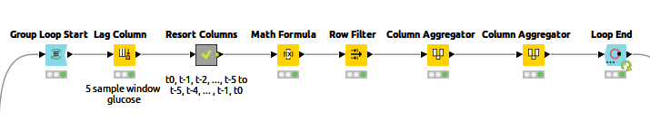
At each iteration, the data of one patient is processed. The Lag Column node in the loop body creates the sequence of n=5 past values of the current column by setting a lag value of 5. The times series produced by the Lag Column node follows this order:

x(t0) x(t-1) x(t-2) x(t-3) x(t-5) x(t-5)

The network needs a sequence in time increasing order, such as:

x(t-5) x(t-4) x(t-3) x(t-2) x(t-1) x(t0)

The “Resort Columns” metanode resorts the sequence appropriately. The output of the Loop End node has the sorted sequences of feature vectors and the corresponding target vectors.

In my example, the input vectors contain samples with three time steps each, while the output has the next three consecutive timesteps. This corresponds to a 15-minute input window and a 15-minute prediction window.

Afterward, the data is split into training and test sets by taking 80% of the data for each patient from the top as training set and the remaining 20% as test set. Keep in mind that since this is time series data, you don’t want to take random samples. Additionally, I did not include "Diabetes_Patient_008" in the training/testing process. This patient will be used for validation purposes.

The Long Short-Term Memory (LSTM) network is a type of recurrent neural network, often used in deep learning because even very large architectures can feasibly be trained with it. It is commonly used for time series prediction.

Instead of neurons, LSTM networks have memory blocks that are connected through layers. A block has components that make it smarter than a classical neuron and give it a memory for recent sequences. I won’t go into detail, but if you are interested, read this great blog post about LSTMs.

The network I used consists of five layers, as seen in Figure 4.

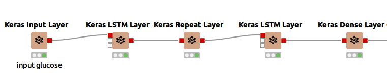
The five layers in detail:

1. An input layer to define the input shape implemented via a Keras Input Layer node. The input shape is a tuple, represented as n, m, where n is the length of the sequence and m is the size of the feature vector at each time step. In this example, the input shape is 3,1 (three time steps of 5 minutes and one feature (glucose level)).

2. An LSTM layer implemented via a Keras LSTM Layer node, using 100 units (length of the vector in hidden state) and "ReLu" as its activation function.

3. A Repeat Layer that repeats the input three times. The Repeat Layer adds extra dimensions to the dataset.

4. A second LSTM layer using 100 units and "ReLu" activation function. This time the "Return sequences" option is enabled (this returns the hidden state output for each input time step).

5. A Dense Layer that connects each unit of the layer input with each output unit of this layer. This generates an output of the shape 3,1 (like the input shape)

Using a Keras Network Learner node, the created model can be trained. I trained the model for 100 epochs, and then used the Keras Network Executor on the test and validation set.

To view the results, I again created an interactive view, which makes it possible to select the different patients and plot the corresponding result. Figure 5 shows an example result for “Diabetes_Patient_001."

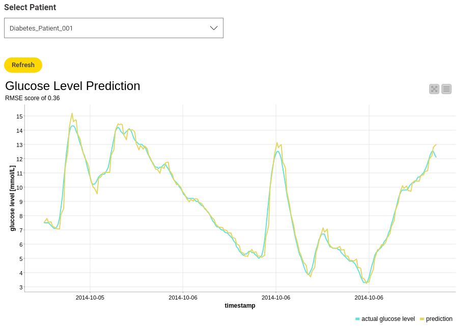
The Root-Mean-Squared-Error (RMSE) score is 0.36, which is pretty good and means that the difference between the actual and predicted data is not that big. This can also be seen in the line plot, showing the actual and the predicted glucose values.

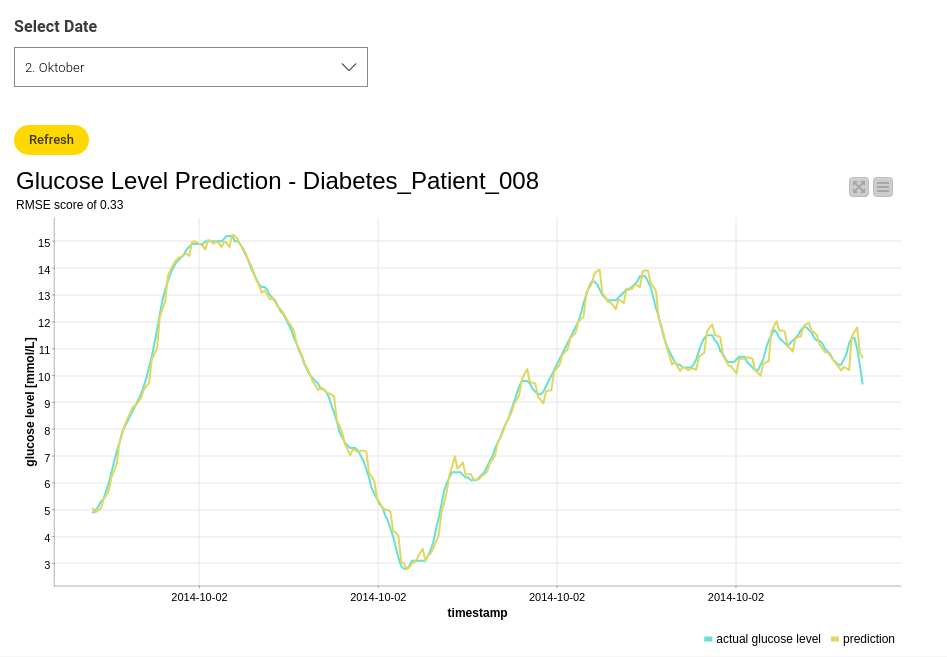
Let’s see if the results also look this good by using the validation data. I used "Diabetes_Patient_008" for this. Figure 6 shows the actual and predicted glucose values for "Diabetes_Patient_008" on October 2nd. You can select different dates to make the view more clear, but the overall RMSE value for the validation data is 0.33. Pretty good!

If you want to see more results, check out the workflow and play around with it yourself. Now that it’s been trained and tested, the model can be deployed for further purposes.

CGMs can do a lot to help someone keep track of their blood glucose levels during the day. Future blood glucose predictions can help even more. With this, diabetic people could, for example, estimate whether they’ll need insulin in the next 15 minutes. In this post, you saw how a Many-to-Many LSTM network can be used for such predictions. Check out the Digital Healthcare space on the KNIME Hub for more workflows to download and use yourself. Thanks for reading!