How to take control of data drift

This is the second part of our journey into model monitoring with an anomaly detection approach. In a previous blog post, we described how this approach needs simulated data, and showcased a solution to generate some. Today we are using that simulated data to introduce the model monitoring application. The workflows described in these posts are available on the KNIME Hub.

Real data is not always kind. In this interview, data science expert Dean Abbott talks about how COVID-19 changed the data our models were trained on, and how the models have struggled to adapt to the new reality: “The ‘after’ is different from the ‘before,’” he explains.

In Dean’s example, data shows an unexpected behavior after an exceptional event. In those cases, the discrepancy is easy to pinpoint. However, changes could also be spread out over time, with slight changes happening in the same direction over and over, but not drastically enough to capture our attention unless we take a look at the big picture.

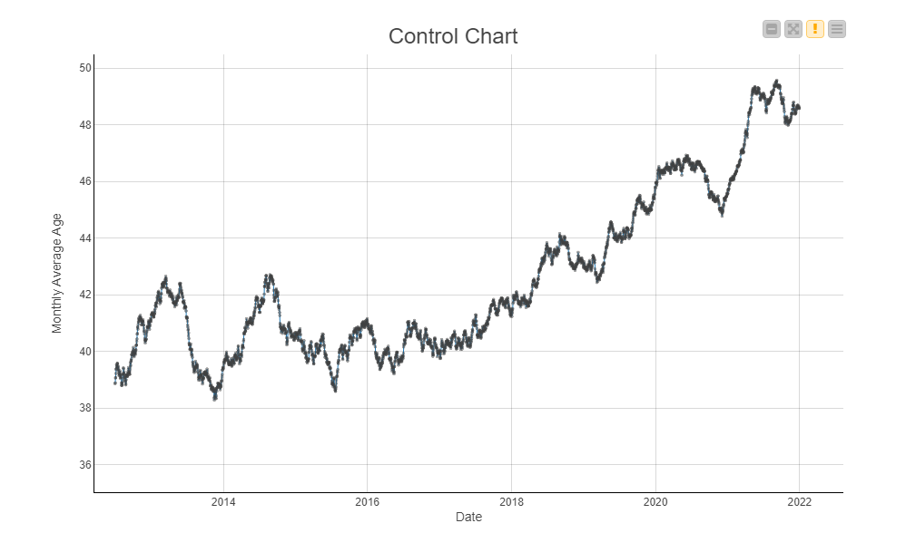
It doesn’t take a pandemic to propagate such a scenario. In Figure 1, the plot depicts a gradually increasing mean for deployment data, representing the age of customers. How do you think a model trained with historical data would behave today? Would it be as effective as it could be? Probably not.

Data changes, and models become outdated and must be retrained with the new data. But when is the best time to retrain a model? And how often should we retrain, given that this is an expensive process?

We have to keep an eye on the changes and make decisions accordingly. Luckily, this whole process can be automated in many ways. In this blog post, we will present a solution for automated model monitoring that leverages the statistics of the deployment data to detect drift.

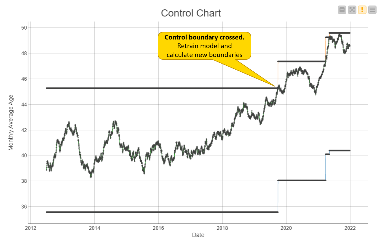
Figure 2 summarizes this process over time. It shows the same drifting data from Figure 1, together with the control boundaries. Thanks to them, our system was able to recognize that the data has exceeded the range of normal fluctuation. The model’s time has come, so it must go off for retraining.

Our final goal is to automatically have a Boolean answer to the question “Does the model need retraining now?” Instead of asking this question by monitoring the model directly, we ask the equivalent question: “Has the data drifted from normal behavior?” We answer this by sending data regularly for checking.

Before digging into technicalities, we set a first level of abstraction. In our use case, we want to check the data on specific columns daily. To do that, we build an initial workflow that determines which column to test and on which time frame — the previous 6 months, in this instance — and returns a flag True or False which indicates the need for retraining. Ideally, this workflow would produce the retraining flag regularly — for example, by scheduling its execution on a KNIME Server.

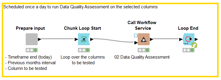
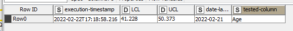
The workflow in Figure 3 accesses the parameters and delegates a second workflow for the actual calculation. Together with the retraining flag, a human-readable message summarizes what is going on under the hood of the data testing (Figure 4).

Using the Call Workflow Service node in the previous workflow, we are able to abstract the technical complexity of the data quality assessment pipeline. Let’s now dig into the technicalities encapsulated in the second workflow which produce the retraining flag.

The called workflow accesses the data to test together with the boundaries, which are stored in an external file from previous executions. Then it performs these two steps:

• Data Quality Assessment: Given the data for the considered period, it contrasts its control statistics with the provided boundaries. The component provides a retraining-flag with value 0 if the data statistic is out of bounds, 1 otherwise.

• New Boundaries Calculation: Carries out the calculation of the new control boundaries when a model is retrained on new data.

For the data quality assessment in our example, we considered the average age of the population over the last 6 months. This data is provided to the Data Quality Assessment Component. Testing this data finally produces the boolean retraining flag.

The two possibilities at this point are handled by a Case Switch node:

• retraining-flag==0: The most recent data is in line with the expectations, thus the model does not need retraining. The system writes a line in the log file and the execution is given back to the caller workflow.

• retraining-flag==1: In the considered period, the data drifted so much from the expectation that the model is outdated and needs retraining. The retraining of the model itself is beyond the scope of this work, and we assume it is automatically executed by an external additional service. What we take care of in this step is the calculation of the new boundaries, explained in the next section.

Our system detected drifted data. The model is no longer effective, and is retrained. Here we assume that a model retraining involves all the new data collected so far. Therefore, old training and new deployment data are used to train a new performing model. Since the training data changed, the control boundaries used so far are also outdated, being based only on the old training data. The Calculate Boundaries component carries out the calculation of the new control lower (LCL) and upper (UCL) boundaries based on the following rules:

LCL = avg - 0.4*stddev; UCL=avg + 0.4*stddev

Where avg is the moving average age calculated with the backward gaussian method.

The new boundaries are appended to a logging file, and will be used as a reference in the next check.

We designed the system in a modular way. The two core steps described above — data quality assessment and new boundaries calculation — are encapsulated in distinct components that can be easily shared and embedded in new applications.

Deployment data might change over time, and because of that, models become less effective than one would expect. However, today we showcased a system that can regularly monitor the data and ring the bell if it gets out of control. With this information, we know when it is time to dispose of an old-fashioned model and train a new one that is aware of current shifts.

The world changes, and data changes with it. We just have to be prepared and react in time!