
Exploring the Wonders of the GroupBy Node for Aggregations
There are many levels to look at data. Sometimes, looking at just the raw data doesn’t bring out the information we need. Often the operation required to move from one level to the next is aggregation.
Let’s take a dataset of purchase contracts as an example
- The pure list of contracts (the raw data), though informative, does not tell us much about the customer contribution to company revenues, customer shopping habits, or even customer loyalty
- But this information can be easily deducted from the list of sale contracts if we perform just a few aggregation operations. For example the sum of the contract amounts, the number of contracts, and the time range covered by the contract list, respectively
Let’s take a dataset of visitors to a web site as another example
- The pure list of visitors to some pages might be too detailed for us to gain useful information
- But describing groups of people (i.e. aggregating) by means of average age and most frequently adopted digital behavior can tell us more
Or again let’s take a technical project and KPIs
- The list of actions requested and performed within the project, in theory describes the cost, impact, and ultimately the success of the project itself.
- But calculating commonly adopted Key Performance Indicators (KPIs), usually involving a few aggregations, makes the picture much clearer for busy project managers
KPIs, aggregation, and professional sports
Another field where KPIs, and therefore aggregation, play a very important role is of course the world of professional sports. Athletes and athletes’ performances are dissected and measured before and after every event. Baseball is the most famous sport for the application of statistics and performance metrics to the players and to the games (Remember Moneyball?). The Olympic games are another area of professional sports where performance metrics are heavily applied and often rely on some kind of aggregation measure.
In general, it is recommended to aggregate data before visualizing it, or conducting statistical analyses. This is important, because the informativeness of these analyses largely depend on the skillful use of aggregation methods.
The aggregation methods covered in these articles
Let’s now explore the power of aggregation metrics, from simple methods – such as counting or sum – to more complex measures – like covariance vs. correlation or median vs. mode.
In this blog post (Part I), we focus on:
Basic Aggregations
- Count vs. Unique Count
- Percent vs. Percent from Unique Count
- Sum
- Range
In the next blog post (Part II), we will focus on:
Statistical Aggregations
- Covariance vs. Correlation
- Measures of Central Tendency
- Measures of Dispersion
The Dataset & the GroupBy node
For this blog post, we will dig into the Olympics Athlete Events Analysis dataset, freely available on Kaggle. It contains comprehensive information on the athletes, sports, and events of the modern Olympic Games from 1896 to 2016. The dataset contains 271,116 rows and each entry refers to the participation of an athlete to one or more editions of the Olympic Games or related sport events, identified by a unique ID and described by name, sex, age, height, weight, Olympic Team, National Olympic Committee (NOC), sport and event in which he/she competed, won medals, game and year of the Olympics, season, and hosting city of the games. Except for “ID” and “Year”, which are numerical attributes, all other 13 attributes are nominal.
To perform a wide variety of aggregation operations, KNIME Analytics Platform offers different native aggregation nodes. The most powerful of all is the GroupBy node (our gold medalist!). This node requires a two-step configuration (Fig. 2).
1. Groups tab
The Groups tab defines the group of data (customers, dates, pages, or whatever else). It requires us to select the column(s) whose values are used to build the groups.
For example, we might want to group by athlete to collect all participation data for each athlete; or by year to measure the general performances at each edition of the games; or by number of gold medals to get the list of all athletes with n gold medals; and so on. We might also want to define groups by combining more grouping criteria, like for example all female/male athletes (grouped by “Sex”) with n gold medals (grouped by “Medal”).
2. Aggregations tabs
Any of the Aggregation tabs sets one or more aggregation methods for one or more selected columns. Notice that different aggregation methods are available for different attributes, depending on their type. This means that available aggregation methods vary if the input column is, for example, a string or an integer.
The three Aggregation tabs – Manual, Pattern based, and Type based – provide different selection options for the column(s). Manual refers to a manual selection process; Pattern Based selects all columns whose name matches a RegEx or wildcard pattern; Type Based selects all columns including specific data types.
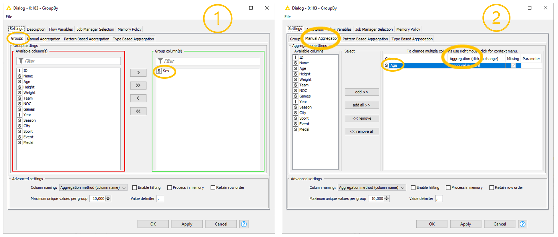
In this blog post we will use the Manual Aggregation tab. While simple, it is sufficient for our demonstration purpose.
Eager learners may find interesting to know that it is also possible to perform grouping without aggregation and aggregation without grouping, just by skipping the corresponding settings in the Aggregation or in the Groups tab, respectively.
On top of the core setting, the GroupBy node offers some advanced settings, shown at the bottom of the configuration window. It is worth mentioning the possibility of including flow variables, changing the column name after aggregation, retaining the row order, and choosing the maximum unique values per group or the value delimiter.
Basic Aggregations – Count, Unique Count, Sum, Range
We will first explore some basic aggregation methods such as count, unique count, sum, and range. Later, as we get more familiar with this node, we will see some more complex statistical aggregations. Right, that’s enough talk. Time to get our hands dirty!
1. Count vs. Unique Count
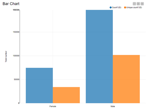
The first insight that we wish to get from our Olympics dataset is the number of male and female athletes who have competed in the Olympic Games since 1896.
To do this, we group the data rows by “Sex” in the Groups tab. In the Manual Aggregation tab, then, we select the “ID” column and the “Count” method. The “Count” method does just that: it counts. It counts all the rows in the group.
Note. “Count” is the only aggregation method that does not depend on the selected column. The number of rows in a group is the same if we count them using the column “ID” or using the column “Age”. This of course is true only if we do not exclude the rows with missing values in the selected column.
The Aggregation tabs of the GroupBy node offer two suitable counting methods: “Count” and “Unique count”. What is the difference?
In each group, we collect all data rows describing participations of female/male athletes to the Olympic games. As we said earlier, some athletes have participated in more than one edition of the Games. However, since they are always the same person, we might want to make sure that we count them only once in the group. “Unique count” enforces the unique counting of distinct data rows. Each athlete is uniquely identified by the “ID” value, and therefore “Unique count” must be executed on the “ID” column. Counting unique IDs automatically excludes duplicates and returns the number of unique male and female athletes.
Results are visualized in Fig. 3. By comparing “Male” vs. “Female” athletes, we see that the total number of male athletes is significantly larger than the total number of female athletes. When we compare “Count” vs. “Unique count”, we see that most athletes have participated in one or more editions of the games or sport event.
Note. Two aggregations methods: “Count” and “Unique count”.
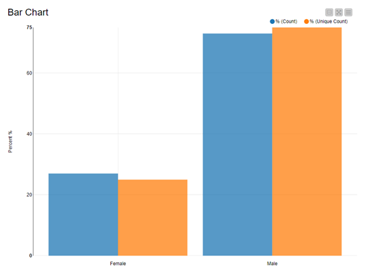
2. Percent vs. Percent from Unique Count
Another way of taking care of duplicates in the “count” method is to use percentages. When using percentages, the number of non-unique female athletes is divided by the total number of non-unique athletes. In the previous bar chart, we see that the number of duplicates is similar for male and female athletes. So, the percentages should be independent (or almost independent) from the problem of duplicates. Let’s see if that’s true and calculate the percentages of male and female athletes counting all participations and counting unique athletes only.
We replicate the same column selection in the Groups and Manual Aggregation tab, but this time we select “Percent” as the aggregation method. Note, that “Percent” calculates the percentage based on “Count”, that is considering all rows in the group, including duplicates.
Since the GroupBy node is missing an aggregation method that computes percentage values for unique rows, we select “Unique count” as the aggregation method in the GroupBy node and then use the Math Formula node to calculate the percentage of male and female athletes as the ratio between each unique count and the total unique count of athletes. We name this measure “% (Unique count)”.
Note. Two aggregations methods: “Percent” and percentages on “Unique count”.
Fig. 4 again compares female vs. male athletes (x-axis) and percentages of athlete participations and percentage of athletes (y-axis). It turns out that percentage of participations is not the same as percentage of athletes. Indeed, there is a slight difference in the two percentage values.
Note. Always make sure that you are including the right objects in your count or percentage!
3. Sum
We now want to slightly increase the complexity of our data aggregation methods to find out how profitable it is for athletes to win medals over time. Unfortunately, our dataset does not contain any information regarding medal bonuses for each won medal, but we can integrate this information in our dataset before aggregating it.
In 2018, the CNBC published an article Here’s how much Olympic athletes earn in 12 different countries reporting a rough estimation of how much money athletes can hope to gain for each won medal. Medal bonus amounts vary across countries and medal worth. Moreover, not every country rewards medal-winning athlete with a bonus.
For the sake of simplicity, we will fictitiously assume that over time all medal-winning athletes have gained bonuses that are equal to the 2018 medal bonus amounts for U.S. athletes, as reported by the CNBC: 37,500 USD for any gold medal, 22,500 USD for any silver medal, and 15,000 USD for any bronze medal. We add this information into our dataset in a new column named “Medal Bonus”.
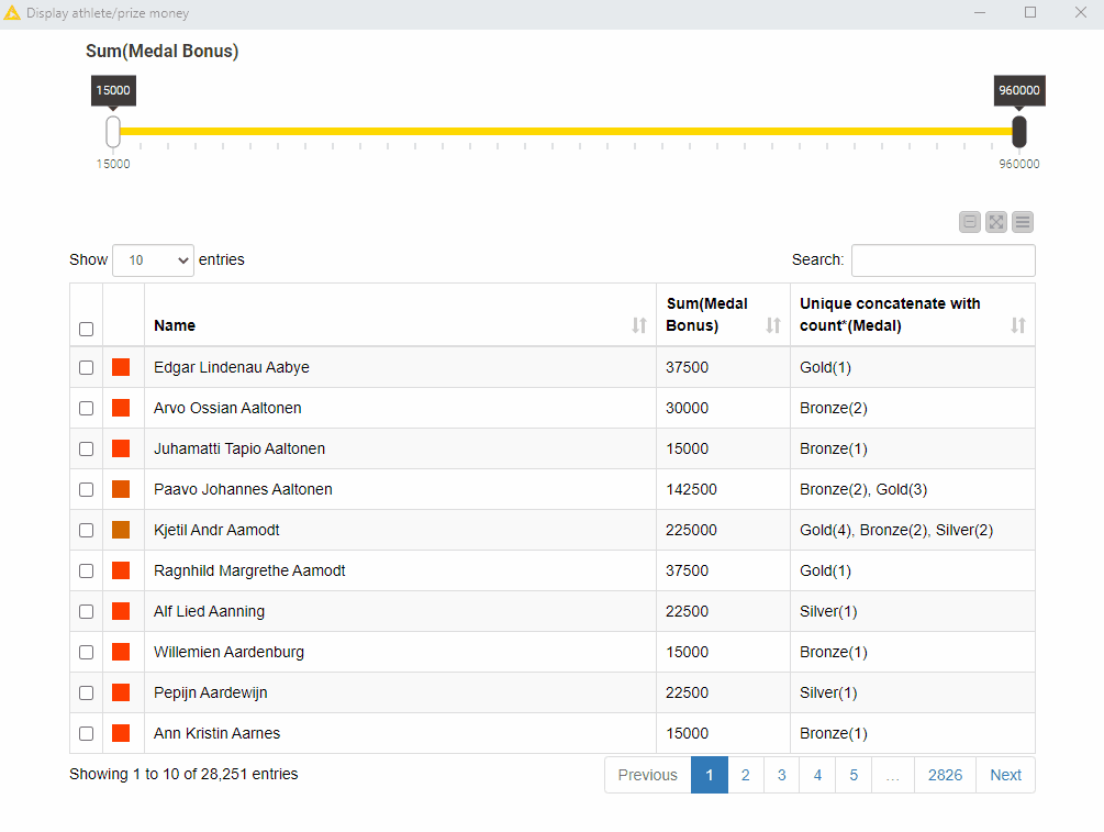
We can now isolate the athletes’ performances, by grouping the data by the attribute “ID”. We also include attribute “Name” in the Groups to carry that on for future visualizations. We then compute the “Sum” over the column “Medal Bonus”.
Moreover, we can include an additional aggregation method, “Unique concatenate with count”, on the attribute “Medal” to find out which and how many medals have contributed to each athlete’s wealth.
Note. Two grouping attributes: “ID”, and “Name”; two aggregating attributes: “Medal Bonus”, and “Medal”; and two aggregation methods: “Sum” and “Unique concatenate with count”.
To visualize our results, we combine a table and a range slider in the final view. The range slider sets the range for the total medal bonus – the sum of all medal bonuses – and the table displays only the athletes – name, total medal bonus, and medal count – within that range. This composite view is implemented in the “Display athlete/prize money” component of the workflow GroupBy: Basic Data Aggregation.
Fig. 5 shows that if we set the lower threshold to 500,000 USD approx., only two athletes fall in that range: Larisa Latynina, a former Soviet artistic gymnast, and Michael Phelps, an American former competitive swimmer.
4. Range
The last basic aggregation method that we are going to explore is “Range”. Range is the difference between the lowest and highest values for a given attribute and applies only to numerical and Date&Time type of columns.
Let’s use this method to check athletes’ career longevity. As a proxy for that, we will calculate the number of years between the first and the last attended Olympic Games.
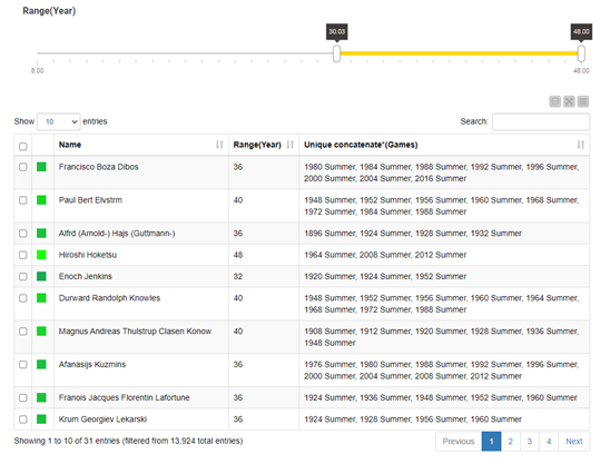
We start by filtering out duplicate rows. We then again use the GroupBy node to group by two attributes, “ID” and “Name”, and compute “Range” on the attribute “Year”.
Optionally, we can also decide to include an additional aggregation method, “Unique concatenate”, on the column “Games” to see the exact list of games in which each athlete has competed.
Note. Two grouping attributes: “ID”, and “Name”; two aggregating attributes: “Year”, and “Games”; and two aggregation methods: “Range” and “Unique concatenate”.
Once again, to visualize our aggregation results, we built a component, displaying a composite view with a range slider and a table.
To get a better feeling for athletes’ career longevity, we arbitrarily set a minimum threshold for range values to eight years (equivalent to three consecutive editions of the Games). That is, we assume that athletes’ career longevity is reflected in more than 8 years of sport activity. It is interesting to notice that applying this threshold also includes athletes who competed in two Games only, but over a very long-time span.
Fig. 6 shows athletes’ names whose career longevity is 30 years or more. It also shows the year and the Olympic Games in which each athlete competed. An interesting insight is that a couple of athletes have a career longevity of 40 years and have participated fairly regularly in many editions of the Games. The only exception is Japanese equestrian rider Hiroshi Hoketsu, who has the longest career, but participated in only three Olympic Games.
Summary
In this article, we have explored a few basic aggregation measures. What they all have in common is that they are all calculated with one GroupBy node.
The GroupBy node is a very powerful node and very simple to use. In one tab you select the grouping, in the other tab the aggregation measure. Often underestimated, it actually offers several aggregation methods for numerical (37) and nominal attributes (15) in its Aggregation tabs. It is highly likely that you will find the aggregation operation you need in the list of methods the node offers.
In this blog post, we have taken advantage of the simplicity of its configuration to create one or more basic aggregations on groups identified across single or multiple attributes. Despite their simplicity, these basic statistical measures already allow for an insightful investigation of the dataset.
Now it is your turn to get your hands dirty and use the GroupBy node to reveal the information hidden in your data! Try out the workflow, GroupBy: Basic Data Aggregation, that we have used in this post and that is freely available for you to download and use from the KNIME Hub.
In the next blog post, “Aggregations, Aggregations, Aggregations! – Part II”, we will go one step further and we will show you how to implement more advanced statistical aggregations on a dataset, also using the GroupBy node.