
The low-code and open source KNIME Analytics Platform offers a variety of functionality to work elegantly with date and time formats. In this article, we want to give you some tips to perform different operations with dates as date value, string, and number.
All examples in this article are based on the Superstore Sales dataset which is freely available on Kaggle. This dataset is a collection of retail data of a global superstore over the period of four years (2015-2018). It consists of 18 attributes, where especially the columns ‘Order Date’ and ‘Ship Date’ will be of interest.
You can try out the examples using KNIME. It's open source and free to download.
Convert from String to Date&Time or Date&Time to String
You can do more of this type of operation with more Date&Time-related transformation nodes:
- UNIX Timestamp to Date&Time: transform UNIX timestamp into Date&Time cells
- Legacy Date&Time to Date&Time: convert from an old Date&Time format (time zone was always UTC) to a new format; here you can now specify the time zone (to convert in the other direction use the Date&Time to legacy Date&Time node)
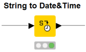
In our Superstores Sales dataset, there are two columns containing date values which are ‘Order Date’ and ‘Ship Date’. But: when reading the data into the KNIME Analytics Platform workspace with the CVS Reader node, the two columns will be parsed as string values. Use the String to Date&Time node to transform the values.
Go to the configuration window (Fig. 2) and first select the relevant columns by moving all the other columns from the Include to the Exclude panel. In our case this is ‘Order Date’ and ‘Ship Date’. Second, select Type and Format. The two columns in our dataset contain only date values in the format dd/MM/yyyy and no time stamp. This indicates to set New type to ‘Date’ and Date format to dd/MM/yyyy accordingly (as shown in Fig. 2).
Tip: Use Guess data type and format to automatically detect the correct data type. It is important to select the correct date format in order to successfully transform the values into Date&Time. Otherwise, the transformed dates might be wrong, or an error occurs.
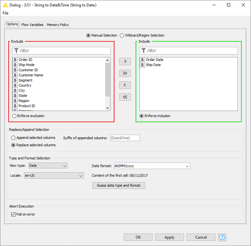
Fig. 2. The configuration window of the String to Date&Time node.
Now we have successfully converted our input to the Date&Time format yyyy-MM-dd (Fig. 3) and can continue with other Date&Time-related operations.
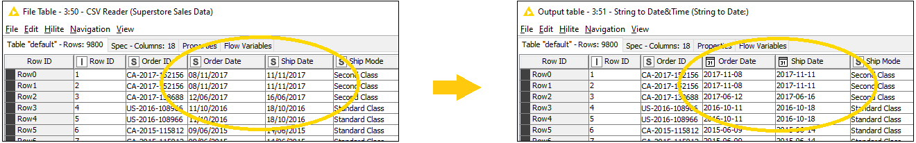
Fig. 3. ‘Order Date’ and ‘Ship Date’ before and after the transformation.
Extract Date&Time Fields
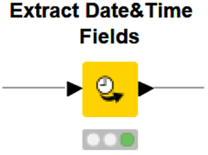
In our example, we could use such fields to find out more about the structure behind the retail data collected. For example, we could inspect the dataset and look for fluctuations in demand. Let’s see how we get this information.
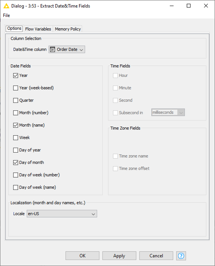
In the configuration window of the node (Fig. 5), we need to select the column of which the Date&Time fields shall be extracted. Note that this only works for Date&Time columns, so you might need to convert the relevant column to Date&Time first. Then you select the fields you want to extract by checking the corresponding boxes. In our example, we extract the Year, Month(name) and Day of month as shown in Fig. 5.
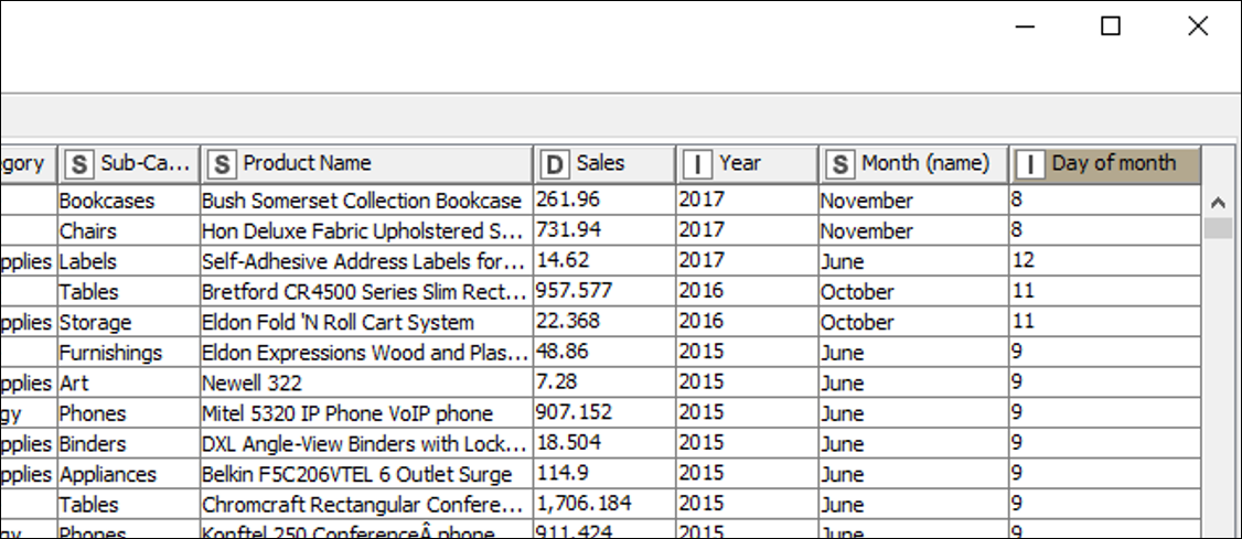
The resulting table is shown in the following (Fig. 6).
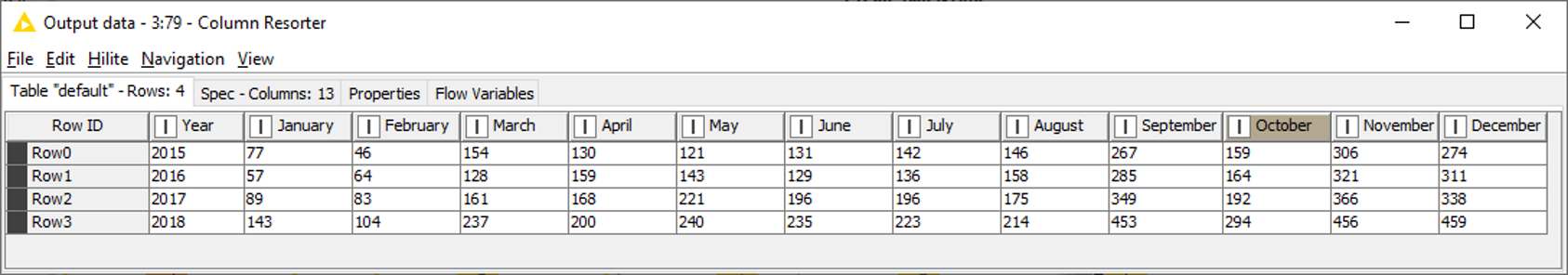
Using the Pivoting node lets us count the number of orders per month and year. Select ‘Year’ as the Group column and ‘Month (name)’ as the Pivot column and then count the entries of the column ‘Row ID’. The resulting table is shown in Fig. 7 and provides a view of the monthly orders for each year. This lets us detect trends in buying behaviour or provide insight into seasonal fluctuations.
If you want to learn more about the GroupBy node and Aggregations in general, check out this article.
Filter based on Date&Time
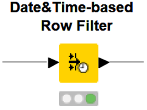
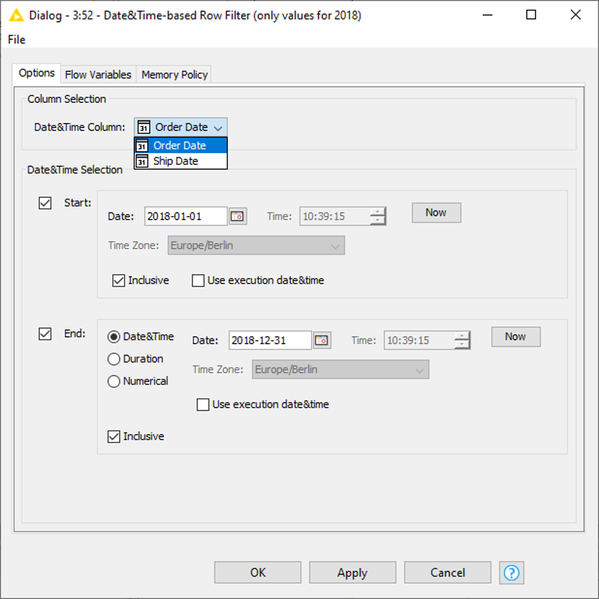
In our example we want to filter on the ‘Order Date’ column and obtain only the data of the year 2018. To apply this filter node, we need to make sure the relevant column is in Date&Time format. Don’t forget to check the box Inclusive in order to include both, the start and end date and make sure to select the correct column (in our case ‘Order Date’).
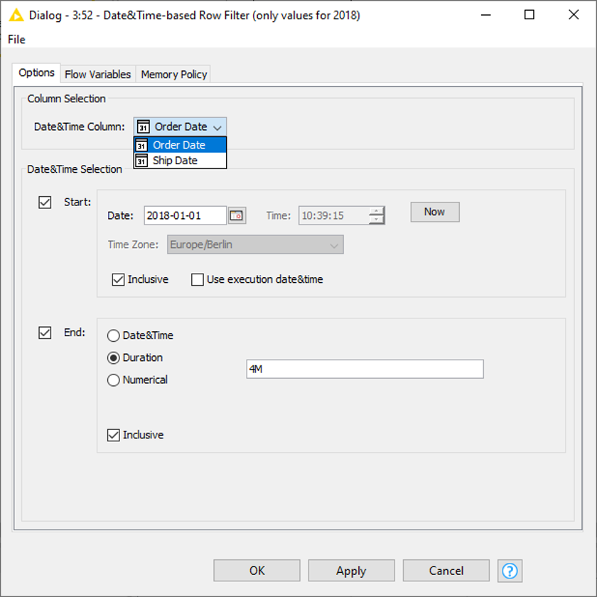
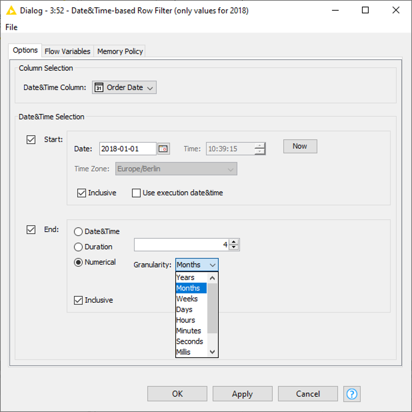
Alternatively, instead of choosing an end date we can define either a duration, e.g., four months (Fig. 10), or enter a numerical value and set a granularity (Fig. 11).
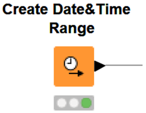
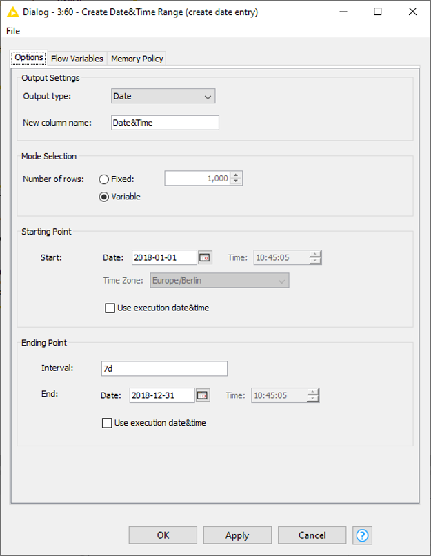
Create Date&Time Range
Imagine, you are only interested in retail data on certain days, then a table as displayed in Fig. 14. comes in handy. With the help of the Joiner node, it can be used to match all Date&Time values of the output table with the entries of the Superstores Sales dataset.
As per the settings displayed in Fig. 13, this node creates a table with only one column containing Date&Time values, starting on 2018‑01‑01 and creating an entry for every seventh day.
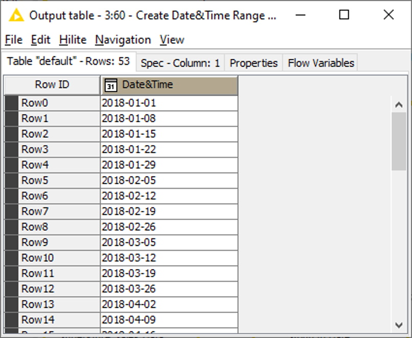
The corresponding table is shown in the following (Fig. 14).
Date&Time Difference

Fig. 15 Date&Time Difference node
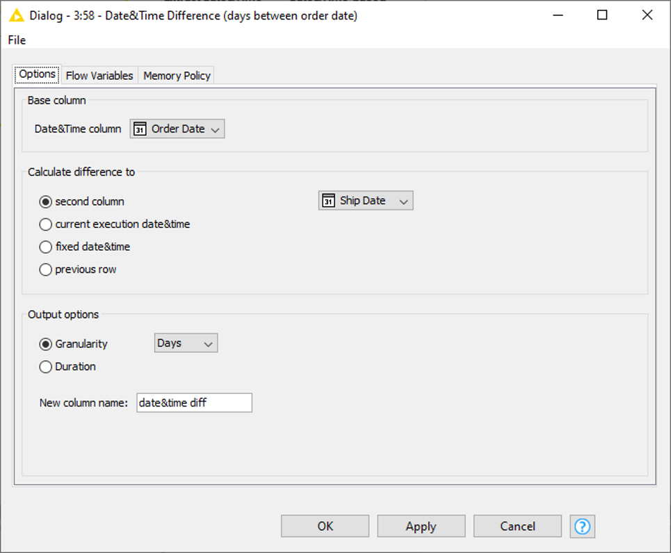
With regard to the Superstore Sales dataset, you might want to use this node to see how much time lies between the ‘Order Date’ and the ‘Ship Date’. In the node’s configuration window (Fig. 16) you need to select the Base column and the date to which the difference shall be calculated. This can be another column (as in our case: ‘Ship Date’), the current execution date, a fixed date, or the value of the previous row. The calculated difference can either be outputted as duration (e.g., 3d) or as a number depending on the granularity (see Fig. 17).
The output table of the node is shown in the following (Fig. 17).
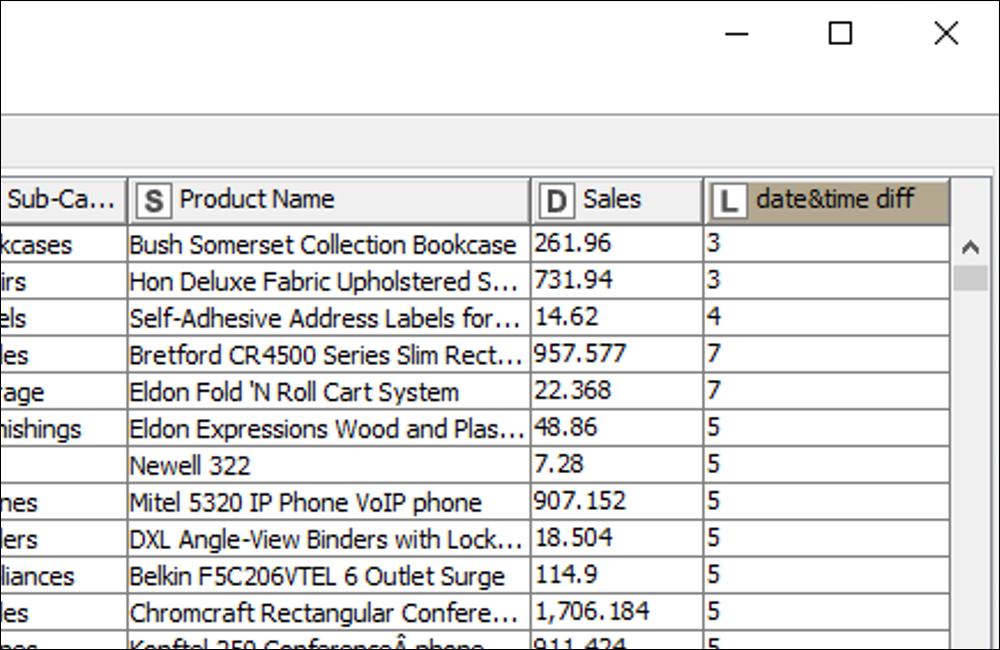
Fig. 17. The difference between ‘Order Date’ and ‘Ship Date’ is appended as a new column to the table.
Date&Time Shift
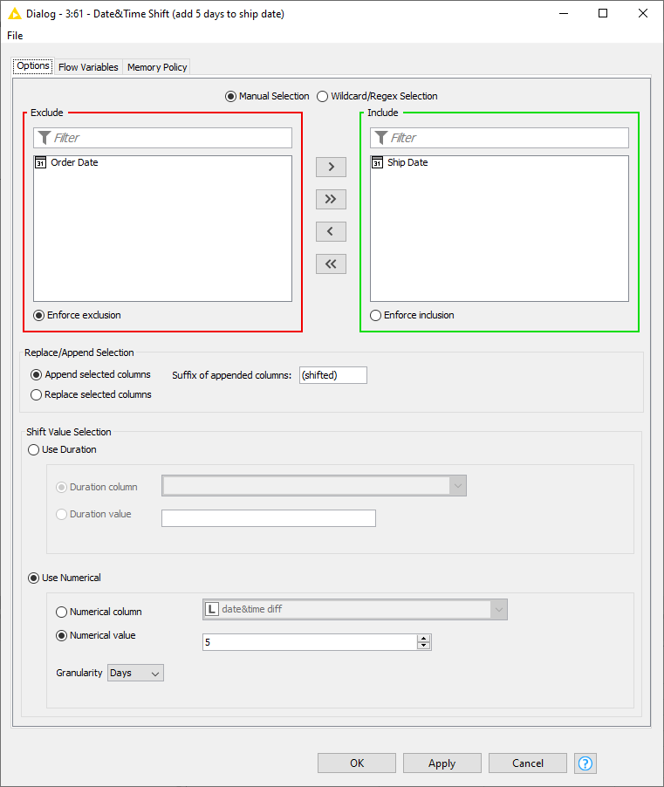
This might be useful, for example, if you want to estimate the delivery date of the shipped goods. Given the information that the shipping process takes 5 days, you can add this time to the ‘Ship Date’ and shift it 5 days. Select the relevant column in the configuration window (Fig. 19) of the node via the Include/Exclude panel. One or more Date&Time columns can be selected. Then define the shift value, in our case 5 days. The column containing the shifted values can either be appended to the table or replace the input column(s).
Extend the Range: The Aggregation Granularity Component for Repeatable Operations
Let’s extend our horizon to use not only nodes but also components. A component is a group of nodes which encapsulates and abstracts the functionalities of this group. Components can have their own dialog and interactive view. They can be reused in different workflows and you are able to share your components with others via KNIME Server or KNIME Hub.

Fig. 20 Aggregation Granularity component
To insert this component into your workflow, locate the item on the KNIME Hub (type ‘Aggregation Granularity’ in the search bar) and drag and drop it into the workflow editor area.
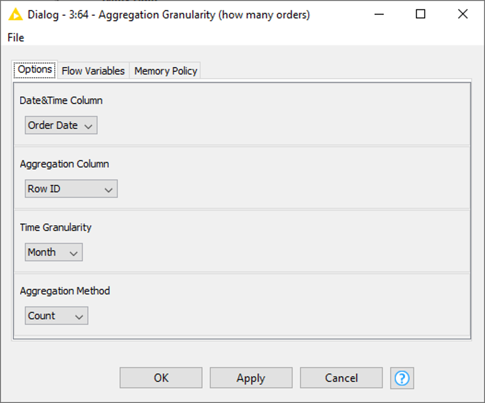
The component generates a table with three columns: the aggregated time stamp, the aggregated values and a constant value column containing the type of granularity. In Fig. 22 you see the resulting table, where the number of orders (column: ‘Row ID’) is counted for each month.
For example, when Quarter is selected as Time Granularity, the component returns the number of orders per quarter.
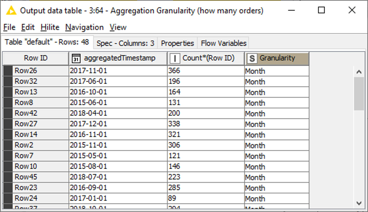
If you have a close look, you can see that the counts of this figure are the same as in Fig. 7, just arranged differently. Thus, the Aggregation Granularity component can be considered as an alternative of the above showed method.
Custom-built Date Formats – Best Practices by Markus Lauber
One of the questions with Date fields is how to store them – either as strings that can be universally stored and loaded, or as UNIX timestamps, or with the internal KNIME format. ‘Real’ date and time columns have the benefit of being able to do calculations and shifts with them; date and times as strings or easy to interpret numbers are easier to store and read back if you deal with systems other than KNIME.
Be sure to always check your results! KNIME helps with the conversion with the UNIX Timestamp to Date&Time node.

For the output you can choose between local and zoned date and time formats and if necessary, add the time zone. (Fig. 23).
With UNIX Timestamps it is essential to see what type they are. They come in seconds, but also milli-, micro- or nanoseconds are possible. So, make sure you check which type you are using and whether your database or target file (other than KNIME) does fully support that format.
In KNIME Analytics Platform the Date&Time format is yyyy-MM-dd. This means, whatever you read into KNIME Analytics Platform, as soon as you transform it into Date&Time cells, it will be in the format yyyy-MM-dd by default.
Sometimes it makes sense to store your data and time variables as ‘readable’ numbers or strings. One way to quickly do this is extract the year month and day from a data and use a math operation to create a date or a timestamp. One way to do this is to extract the year, month, and day as numbers from a date and then for example use the Math Node like this:
(year * 1000) + (month * 100) + day
2021-06-07 => 20210607
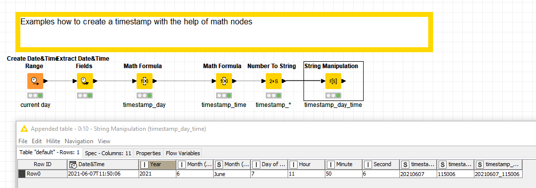
Try this out with the workflow (Fig. 24) Examples how to create a timestamp with the help of math nodes, which you can download from the KNIME Hub.
You could also use the rule engine to manipulate timestamps. This workflow shows Various operations with dates as date value, string and number and demonstrates how to convert from string to Date&Time (format: yyyy-MM-dd) and from there back to string but using the custom format dd-MM-yyyy. Download the workflow Various operations with dates as date value, string and number from the KNIME Hub

Timestamps can come in handy if you want to have versions of your files or want to identify the latest version or store previous ones. Check out this workflow on the KNIME Hub: Examples with timestamps and durations and file names
You could use time nodes and rule engines to create timeslots to aggregate collections of time data into individual blocks. For example to divide an hour into segments of 15 minutes. You can download this workflow Examples how to create a timestamp with the help of math nodes from the KNIME Hub to try out examples.
Also, if you have to do with sometimes messy or complicated date and time formats you can handle them with the help of KNIME nodes even if you have to be somewhat creative. You might combine Date/Time Nodes and Rule Engines for example to handle AM/PM time formats. Download this example workflow Deal with (messy) time formats containing AM/PM distinctions from the KNIME Hub to try this out.Summary
Working with Date&Time values can be tricky. That’s why KNIME Analytics Platform offers specific nodes for Date&Time-related operations. To make use of these nodes, it is crucial to transform the relevant columns into Date&Time cells. In this article, we’ve explained how this is done and shown some of the operations than can be applied to Date&Time cells.
Now it’s your turn! Try out different operations and get used to the Date&Time-related nodes in KNIME Analytics Platform. You can download the workflows used in this article from the KNIME Hub or experiment with your own data.Resources: The example workflows mentioned in this article
- Various operations with dates as date value, string and number
- Examples how to create a timestamp with the help of math nodes
- Various operations with dates as date value, string and number
- Examples with timestamps and durations and file names
- Examples how to create a timestamp with the help of math nodes
- Deal with (messy) time formats containing AM/PM distinctions