
Every 60 seconds, 30,000 minutes of video material are uploaded to YouTube. Hate speech, predatory behavior, graphic violence, malicious attacks, and content that promotes harmful or dangerous behavior is not allowed on YouTube. To check that none of this content is published, YouTube would probably need 90,000 employees, working in three shifts, monitoring the material uploaded every minute.
Today's increasing volumes of video and image data on the one hand and the large variety of use cases in different fields on the other is creating a need for faster, automated execution of computer vision tasks.
Computer vision is a research field that aims to automate tasks performed by our human visual system e.g., detecting different objects in images, semantic segmentation, or neural style transfer. You could say that computer vision enables the computer to see and understand digital images and video, by deriving meaningful information. Convolution neural networks (CNN) are commonly used to derive this information.
Note. This post (a revised version of the article originally published on Low Code for Advanced Data Science) introduces you to the topic of computer vision, gives you an idea of what is behind CNNs for image classification, and shows you how you can implement a CNN using KNIME Analytics Platform, code free.
So let’s start with the question:
Why Use Deep Learning to Solve Computer Vision Tasks?
Deep learning performs much better on computer vision tasks than traditional approaches. This can for example be seen by looking at the winners of the ImageNet Challenge, where the goal is to classify images into 200 classes. Figure 1 shows the performance of the winning model.

It shows a big performance improvement starting from 2012, where deep learning models started to win the competition.
Before taking a look at the idea behind these winning models, we need to understand how a machine sees images.
How Does a Machine See Images?
A machine only understands numbers. Therefore we need a numerical representation for images. A grayscale image can be stored as a matrix, where each cell represents one pixel of the image and the cell value represents the gray level of the pixel.
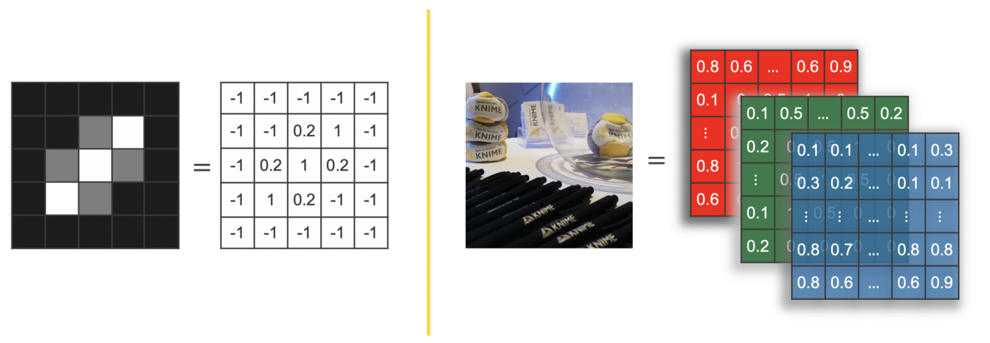
For example, the grayscale image on the left in Figure 2 with size 5 x 5 pixels, can be represented as a matrix with dimensions 5 x 5, where each value of the matrix ranges between -1 and 1. -1 for a black pixel, 1 for a white pixel, and a value in between for any other level of gray.
For color images more than one value is needed to define the color of each pixel. One option is to use the RGB code i.e., the three values specifying the intensity of red, green, and blue in the pixel color. In this case a tensor with three channels is used to represent the image.
Now that we are familiar with the numerical representation for images, let’s think about a good network architecture for image classification and let’s try to start with a feedforward neural network to understand why we need a special architecture when it comes to image data.
Why Do We Need Special Networks for Images?
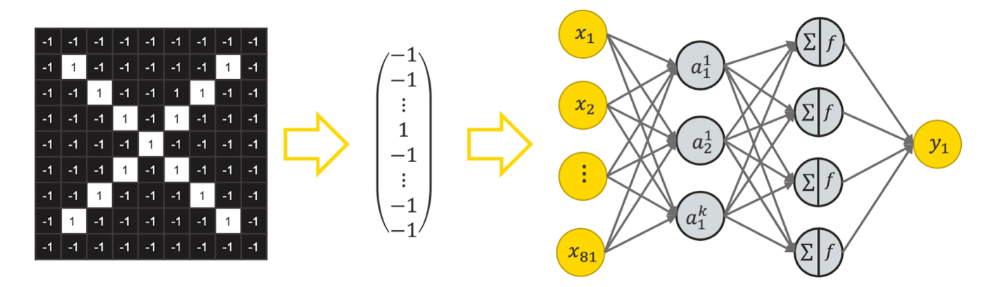
Let’s try to apply a fully connected feedforward network for image classification. To do so, we could flatten the tensor to represent an image with a vector and feed the vector into a feedforward neural network, as visualized in Figure 3.
This raises two problems:
-
Too many weights. A network like this would have a lot of weights. For example, a feedforward network for a colored image with 224 x 224 pixels with 100 units in the first hidden layer, has 224*224*3*100 = 15 052 800 weights only in the first layer. This is unmanageable to train and likely leads to overfitting.
-
Loss of spatial dependencies: In the flattening step we lose all spatial dependencies, which are actually important.
So, we need some kind of other network structure for image data.
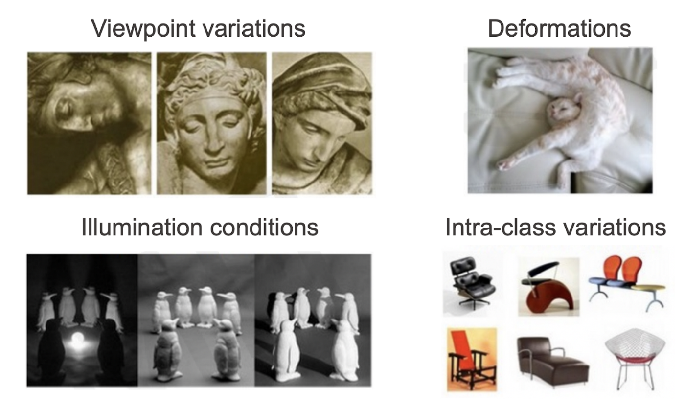
Another challenge when it comes to image classification are the different variations of the same object e.g., different illumination, different size, different viewpoints, different types of the same object, etc.
A network architecture that solves these issues are convolutional neural networks.
What is the Idea Behind a Convolutional Neural Network for Image Classification?
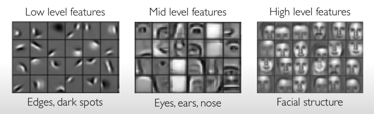
The idea of convolutional neural networks (CNN) is to extract a hierarchy of features, checking for these features in different image patches. The first layers may detect low level features like edges and dark spots, which are then used to extract mid level features like eyes, ears, and noses, which, in turn, are used to detect high level features like facial structures. Using only image patches and a hierarchy allows us to handle different variations of the same object.
But how can we detect whether a certain feature is in an image patch or not?
How Can We Detect Features in an Image?
To detect whether or not a feature is in an image patch we can use a filter. A filter should produce a
-
High value if the feature is in an image patch
-
Low value if the feature is not in an image patch
The key behind a filter is a kernel, which for grayscaled images is a matrix, for colored images a tensor with as many color channels as in the image. Let’s consider the grayscaled case.
To check whether or not a feature is in an image patch, the kernel is placed on top of an image patch. Then the values that lay on top of each other are multiplied. Afterwards all terms are summed up. This operation is called a convolution and produces a high value if the feature is in an image patch and low value if it is not.
In the deep learning community this operation is called a convolution and is represented via an asterisk ∗. Strictly mathematically speaking it is a cross correlation.
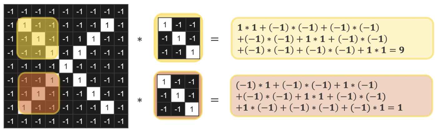
Figure 6 shows you an example. The used kernel checks whether or not an arm of an x going from the upper left to the lower right is in an image patch. If the filter is applied to an image patch which has such an arm (upper part in yellow), the convolution results in the value 9. On the other hand, if it is applied to an image patch where we actually have an arm going in the opposite direction (from the lower left to the upper right) it results in the lower value 1.
To find out in which area of the image we have an arm going from the upper left to the lower right, the kernel needs to be applied to each image patch of size 3 x 3. Therefore, the kernel is moved across the whole image e.g., by starting on the upper left corner and then moving the kernel always one pixel to the right until we reach the right hand side, then one pixel down starting again from the left to right. The resulting matrix is called the feature map. It tells us in which part of the image the feature is present.
One approach to solve the task of image classification is to use domain knowledge to define important features and to handcraft kernels that detect these features. Handcrafting these kernels is hard though, considering that they need to take into account all variations of a feature.
The solution is convolutional neural networks, where convolutional layers learn which features are important and which kernels are necessary to detect them.
How Does a Convolutional Layer work?
As the name of the layer indicates, the convolutional layer also uses the convolution operation as described above, with one additional step. After calculating the convolution for an image patch, an activation function is applied e.g., ReLU. Like in the example of the manual filter above, the kernel is moved across the image to create the feature map.
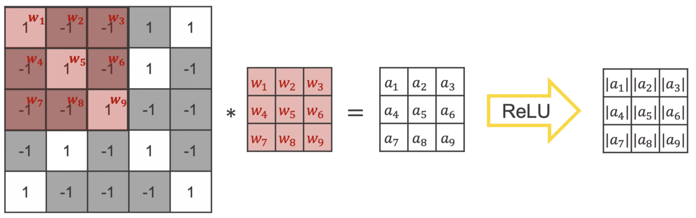
The values of the kernel are the weights of a convolutional layer. This means, during training the convolutional layer learns which features are important and which values a kernel needs to detect them.
 Figure 8: Configuration of the Keras Convolution 2D Layer node.
Common setting options in a convolution layer are:
-
The number of filters that are trained in one layer
-
The size of the kernel defined via a tuple e.g., 3, 3
-
The stride, which defines how many pixels the kernel moves between two convolutions
-
Whether to use zero padding before applying the convolutional layer
-
The dilation rate used for dilated convolution, taking into account not every input value, but for example only every second (dilation rate = 2,2)
-
Activation function
In KNIME, a convolutional layer can be implemented via a Keras Convolutional 2D Layer node. Via the configuration window you can define all the settings.
Another layer type that is commonly used in convolutional neural networks is the pooling layer.
What is a Pooling Layer?
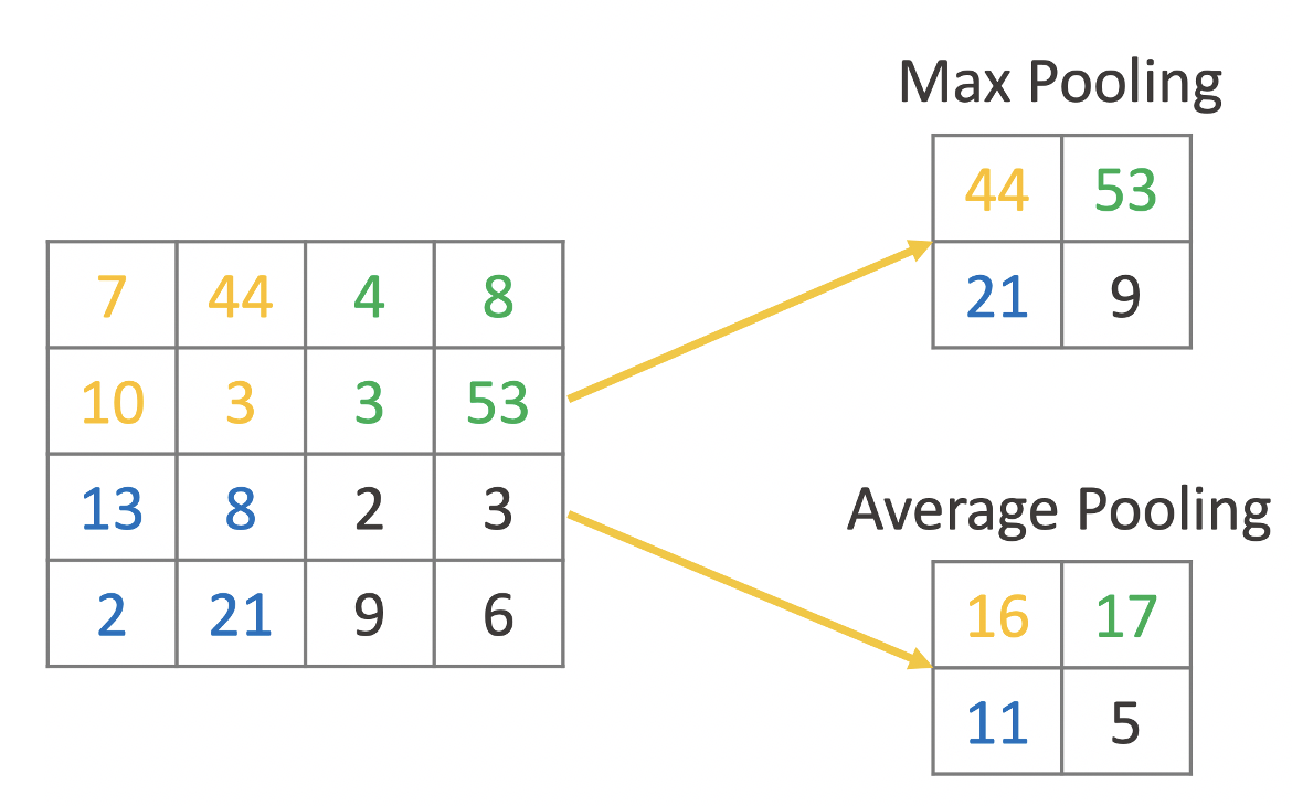
The idea of a pooling layer is to replace areas of an image or the feature map with a summary statistic. The most commonly used statistic is the maximum value, which leads to Max Pooling. Another option is the average value of all values in the area of the image, which leads to Average Pooling. Figure 9 shows an example for both approaches.
Pooling layers are often used in between convolutional layers to summarize the area of an image and to reduce computational complexity.
Let’s now combine everything we’ve learned and train a convolutional neural network for image classification based on the example of the MNIST Fashion dataset.
Implementing a CNN for Image Classification
A CNN for image classification usually has two parts, which are trained together. First multiple convolutional and pooling layers stacked on top of each other, to learn a hierarchy of features, followed by a fully connected feedforward neural network for the classification task. The two parts are linked via a flattening layer which converts the resulting feature map into a vector.
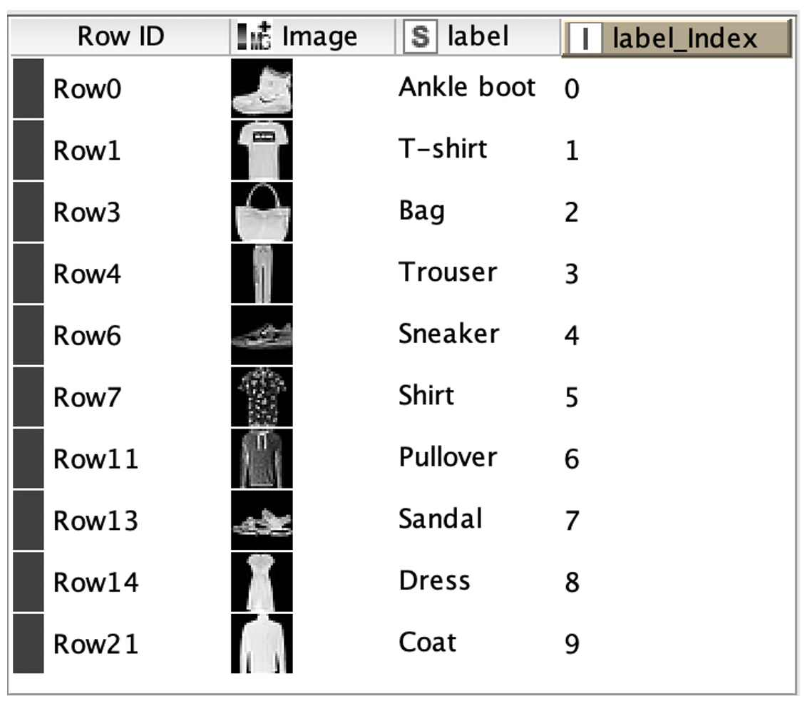
Our goal is to define and train a network implementing this idea for the MINIST fashion dataset. The dataset consists of gray-scaled images of size 28 x 28, which are categorized into 10 different classes.
The screenshot in figure 10 shows you a subset of the dataset including a column with the index encoded label.
The workflow in figure 11 covers all steps from reading data until applying the trained network to some test data using the Keras Integration of KNIME Analytics Platform.
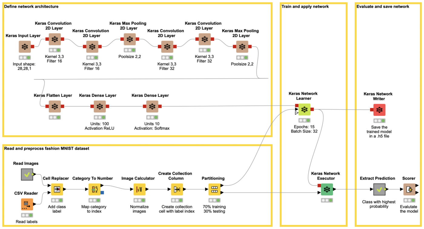
Step 1: Define the Network Architecture
The workflow starts on the upper left with the definition of the network architecture. In the example the following architecture is used:
- A Keras Input Layer to define the input shape in this case 28, 28, 1
- A combination of 6 Keras Convolution 2D Layer and Keras Pooling 2D Layer nodes for the feature extraction
- Keras Convolution 2D with 16 filters, a kernel size of 2,2 and a stride of 1,1
- Keras Convolution 2D with 16 filters, a kernel size of 2,2 and a stride of 1,1
- Keras Max Pooling with pool size 2,2 and stride of 2,2
- Keras Convolution 2D with 32 filters, a kernel size of 2,2 and a stride of 1,1
- Keras Convolution 2D with 32 filters, a kernel size of 2,2 and a stride of 1,1
- Keras Max Pooling with pool size 2,2 and stride of 2,2
- A Keras Flatten Layer node to convert the feature map into a vector
- Two Keras Dense Layer nodes, implementing a hidden layer with 100 units and activation ReLU and an output layer with 10 units and activation function softmax.
Note. A dense layer with activation softmax and with as many units as different classes is commonly used as output layer for multiclass classification. It allows us to interpret the output as the probability of the different classes. For this approach the different classes must be encoded as one-hot vectors, during training.
Step 2: Read and Preprocess the Data
The lower left part of the workflow reads the gray-scaled images of the MINST fashion dataset, adds the label information, performs preprocessing steps like normalizing the images, mapping each label to an index, and partitioning the data into a training and a test set.
Note. The Create Collection Column node converts the label index into a collection cell. This allows the Keras Network Learner node to convert the index values into one-hot-vectors during training.
Step 3: Train the Deep Learning Model
The defined architecture is trained with the Keras Network Learner node.

In the configuration window you can define:
-
The Loss function, in this case Categorical Cross Entropy.
-
The columns with the input for the network, in our case the image.
-
The target column, in our case the collection cell with the index encoded class label.
-
The training settings like, epochs, batch size, and optimizer.
Step 4: Apply and Save the Trained Deep Learning Model

With the Keras Network Executor node the trained model can be applied to the test set and to new data.
With the Keras Network Writer node the trained model can be saved as an .h5 file and used during deployment, either by another workflow or via a coding language that supports Keras models, e.g. Python.
Afterwards the class with the highest probability is extracted and the model is evaluated. With the defined network and training parameters the deep learning model reaches an accuracy of 92%. Want to try it out? Download the example workflow from the KNIME Hub.