The ability to effectively automate tasks normally performed by humans for processing large amounts of image and video data is the ultimate goal of computer vision research.
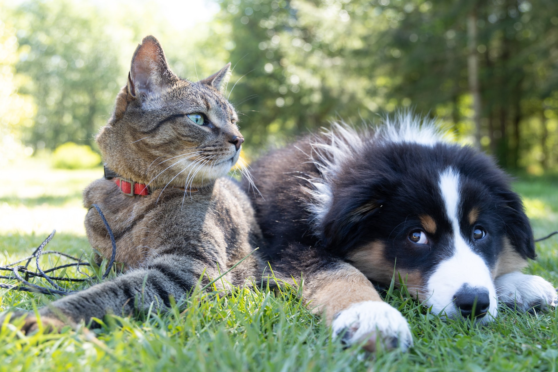
Image classification is used in computer vision to classify whether a certain object or pattern is an image. This technique is used for example in marketing analytics as the first step in analyzing images viewed by a website visitor, in life sciences to aid in disease diagnosis, or in manufacturing analytics to detect cracks or other quality issues in mechanical products.
Approaches for image analysis come in different flavors and levels of complexity, from simple processing to AutoML-based web services. In this post, we are going to define a Convolutional Neural Network (CNN), then train and deploy it for the classification of dog and cat images in KNIME Analytics Platform using the KNIME Deep Learning - Keras Integration. CNNs have proved superior at automatically analyzing and extracting key image features.
The training and deployment workflows described in this article are available for you to download for free on the KNIME Hub. The Machine Learning and Marketing space on the KNIME Hub contains example workflows of common data science problems in Marketing Analytics. The original task was explained in: F. Villarroel Ordenes & R. Silipo, “Machine learning for marketing on the KNIME Hub: The development of a live repository for marketing applications”, Journal of Business Research 137(1):393-410, DOI: 10.1016/j.jbusres.2021.08.036. Please cite this article, if you use any of the workflows in the repository.
Convolutional Neural Networks in a Nutshell
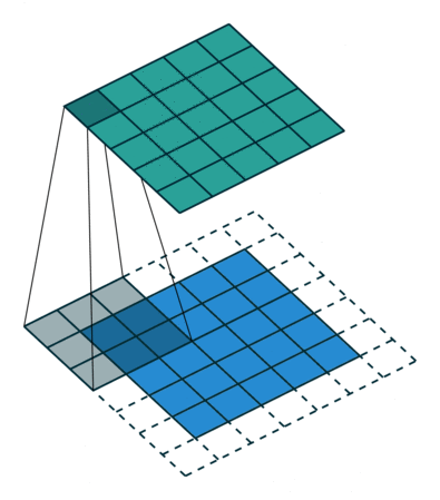
A CNN is a multilayered feed-forward neural network with at least one Convolutional layer (Fig. 2). Convolutional layers automatically extract features from images. To do so, they use a set of kernels, also called filters. Each kernel is a matrix or tensor of weights, customized for the task of extracting a certain feature and learned during the training process.
To apply a filter and extract features, the kernel, which is much smaller than the image, is placed on top of an image patch. The kernel slides over the entire image from patch to patch according to a set of hyperparameters:
-
The kernel size, which is defined via a tuple like 3, 3
-
The stride, which is the number of pixels by which we slide the kernel. If the stride is 1, the kernel moves one pixel at a time.
-
The dilatation rate. Usually kernels are contiguous, but it’s possible for them to have spaces between each cell, called dilation. If the kernel takes into account every second pixel, the dilation rate is 2, 2.
As the kernel is moved across the image, a convolution operation is performed between the kernel and the pixel values (from a strictly mathematical standpoint, this operation is a cross correlation), and a nonlinear activation function, usually ReLU, is applied. This produces a high value if the feature is in the image patch and a small value if it is not (Fig. 2).
To extract a hierarchy of different features, CNNs usually have multiple Convolutional layers stacked on top of each other. Typically the first Convolutional layers learn to extract low-level features like spots and edges. These features are then used by the next Convolutional layer to extract mid-level features — in our case, these would be things like parts of the ears or mouth. The mid-level features are then used to extract high-level features, such as the full representation of cats and dogs.
Other commonly used layers are Pooling layers, for the creation of highly informative feature maps via averaging or max value selection, and Flatten and Dense layers, which are used to define a fully connected feed-forward neural network trained for the actual image classification (Fig. 3).

Read more about Computer Vision and CNNs in Convolutional Neural Network and Computer Vision and A Beginners Guide to Codeless Deep Learning: MNIST Digit classification.
Set up KNIME Analytics Platform for Deep Learning
The KNIME Deep Learning - Keras Integration allows you to define, train, and deploy deep learning models using the Keras libraries in KNIME Analytics Platform. By simply drag-and-dropping the task-specific Keras nodes and connecting them to a pipeline, you can build workflows for your solutions. The KNIME Deep Learning Keras integration is particularly powerful because it combines the ease of the KNIME GUI with the extensive coverage of the Keras deep learning libraries.
To set up your KNIME Analytics Platform for deep learning, you will need to:
-
Set up Python for KNIME Deep Learning.
-
Install the KNIME Deep Learning - Keras Integration.
-
Install the KNIME Image Processing - Deep Learning Extension. This is required only for applications in computer vision.
Additionally, to ensure workflow portability across different OS, it is recommended to use the Conda Environment Propagation node to automatically create a dedicated Conda environment with all the needed dependencies.
Ingest and Preprocess Image Data
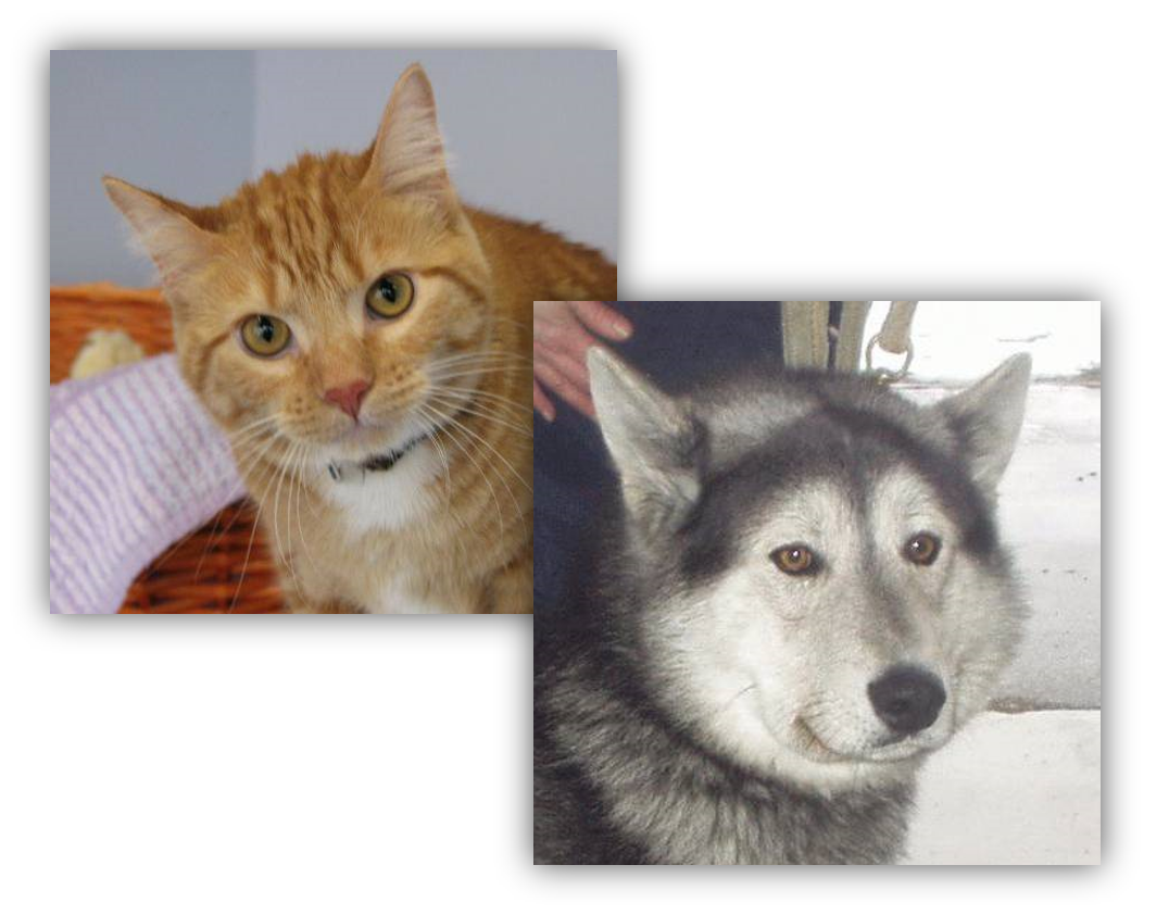
The goal of our article is to build a binary classifier that is able to distinguish between cats and dogs images. To train the classifier, we rely on a Kaggle dataset with 25,000 annotated images, representing cats and dogs equally. The closer the predicted class is to the ground-truth annotations, the more effective our classifier is.
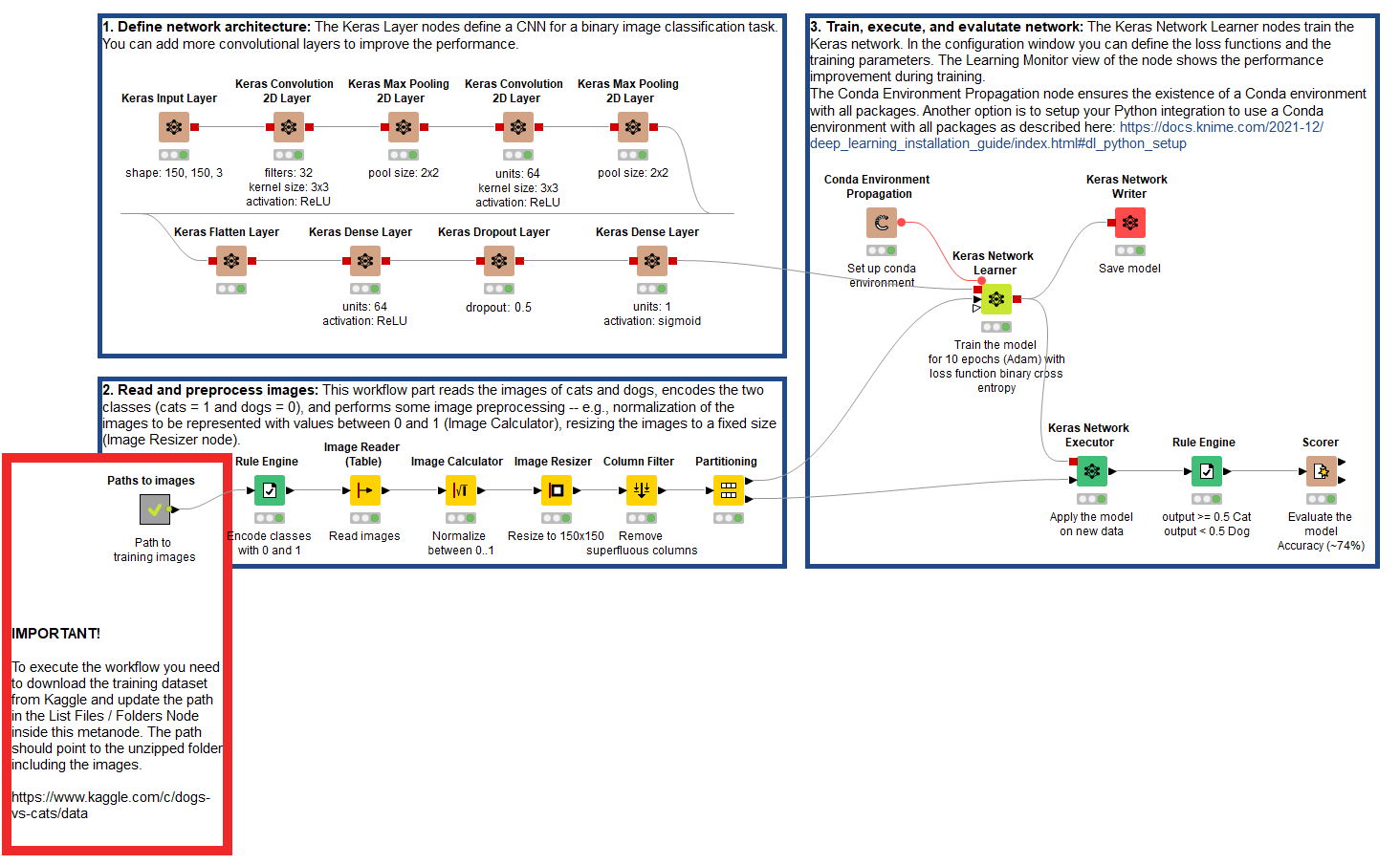
We read the file location of our data with the List Files/Folders node and limit our use case to a sample of 4,000 images to ease the computational burden. Next we use the Rule Engine node to match the strings “cat*” and “dog*” in the file path and encode the target classes as 0 = cat and 1 = dog.
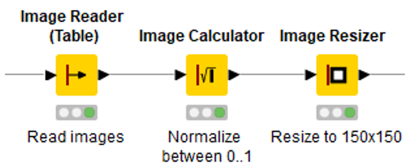
Thanks to the KNIME Image Processing extension, we use the Image Reader (Table), Image Calculator, and Image Resizer nodes to ingest images in a table format, normalize pixel values to fall in the range between 0 and 1, and resize image dimensions to 150x150 (Fig. 4). Minimal preprocessing steps are enough for our use case, but additional manipulation and/or image augmentation techniques might be needed, depending on the task and data at hand.
Define a Codeless CNN
Defining the architecture of a CNN in KNIME Analytics Platform is very simple with the nodes of the Keras integration (Fig. 5). Notice how the codeless network architecture mimics very closely that of Fig. 3: an input layer, Convolutional layers (x2), Max Pooling layers (x2), and a bunch of nodes to define a fully connected feed-forward neural network.
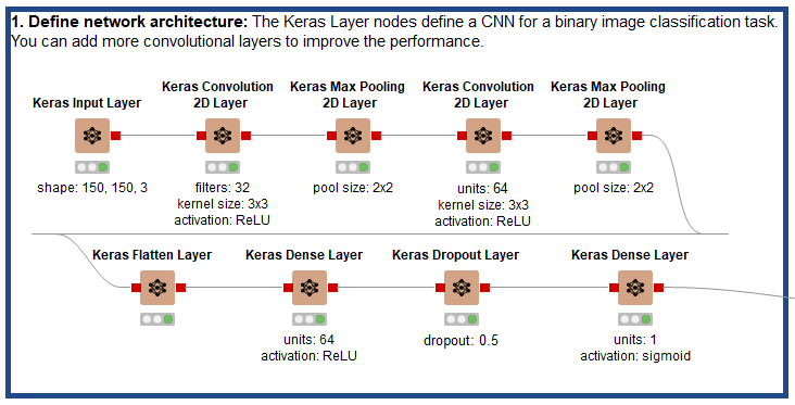
Input Layer
We start by specifying the shape of our input images. To do so, we use the Keras Input Layer node and provide a tuple of integers referring to the image size and the number of channels (Fig. 6). By default, in the “Data format” dropdown menu, the node sets the number of channels at the end, but this can be changed to be in the first position of the tuple if the image shape is different.
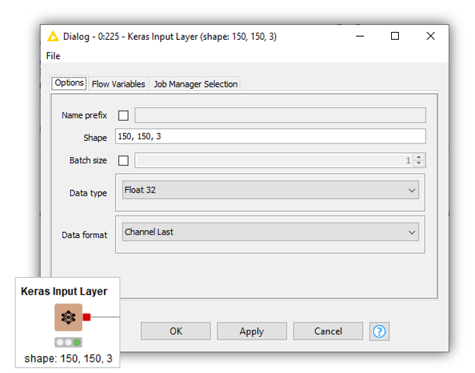
Tip: Use the Image Properties node to find out the shape of your image.
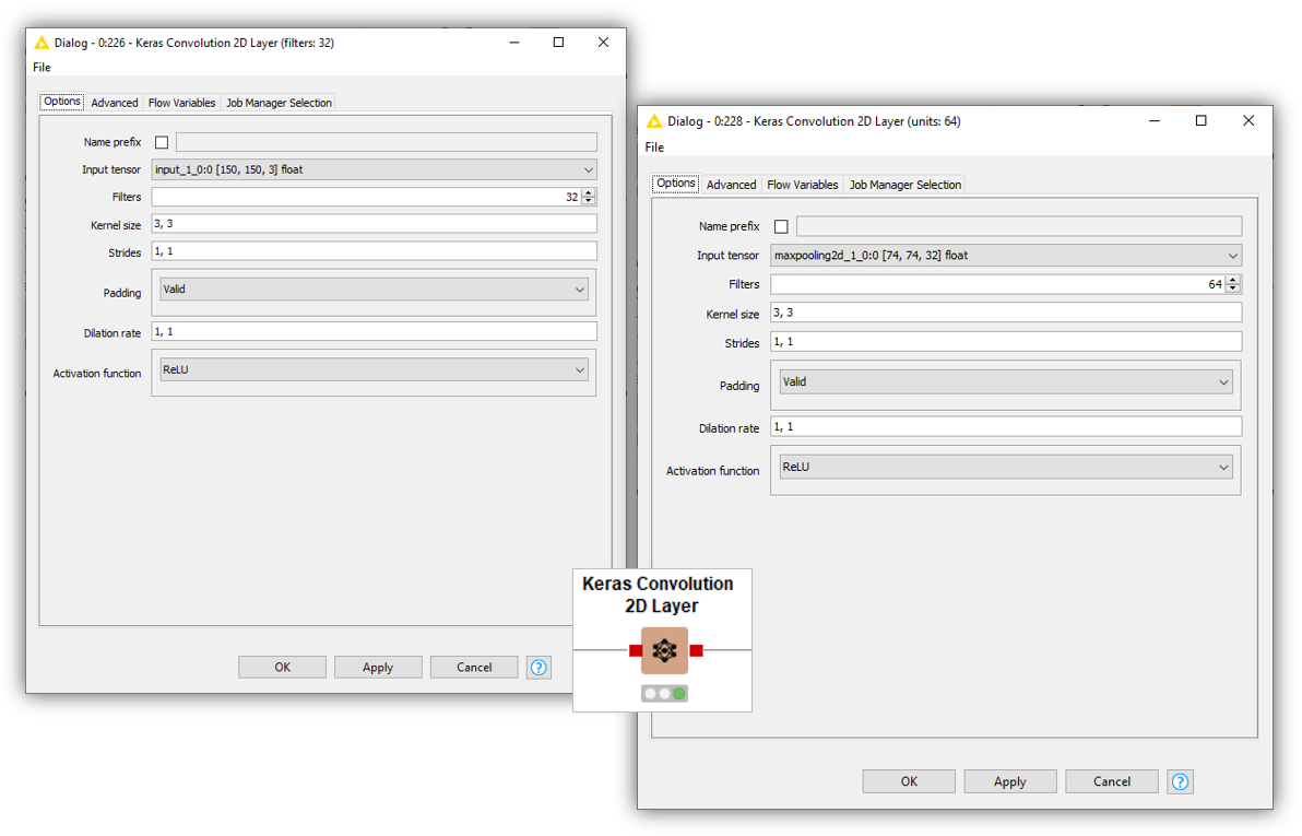
Convolutional Layer
At the core of any CNN lies a series of Convolutional layers. For our use case, we stack two Keras Convolution 2D Layer nodes with similar configuration values (Fig. 7). Indeed, kernel size, stride, and dilation rate are the same. As an activation function, we choose ReLU, but other options (Sigmoid, Tanh, etc.) are available. Additionally, in both cases, we avoid using padding by selecting the option “Valid.” The most important difference is in the number of filters used for feature extraction.
Notice also that in the first Convolutional layer (left), the input tensor has the shape of the input images, whereas in the second Convolutional layer (right) the input tensor has smaller dimensions as a consequence of the Max Pooling layer. It does not display the number of channels in the last position, but the number of filters used in the previous Convolutional layer.
Tip: Learn more about Convolutional layers and their different dimensions in this Data Science Pronto video, What are Convolutional Neural Networks?
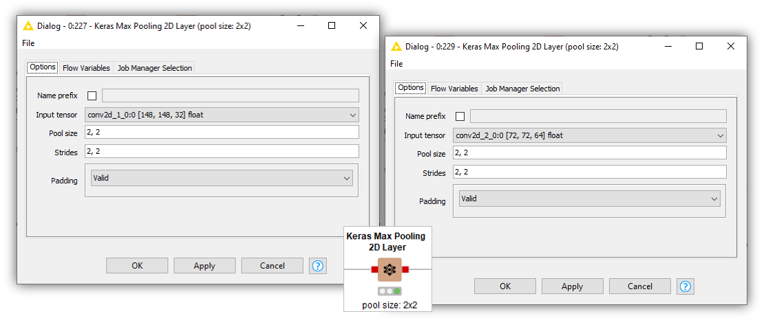
Max Pooling Layer
Stacked between Convolutional layers, CNNs use Pooling layers in different flavors: Max Pooling, Average Pooling, or Global Average Pooling. In our implementation, we use two Keras Max Pooling 2D Layer nodes with the exact same settings. The key configuration is the “Pool size,” which refers to the size of the pooling window in two dimensions. Notice as well how in this case the input tensor changes after each Convolutional layer.
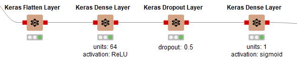
Fully Connected Feed-forward Neural Network
The top layers of a CNN define a fully connected feed-forward neural network that is trained for image classification (Fig. 9). In the top part of the network, we stack a few layers:
-
Keras Flatten Layer to convert the feature map into a vector.
-
Keras Dense Layer to implement a hidden layer with 64 units and activation ReLU.
-
Keras Dropout Layer to prevent overfitting.
-
Keras Dense Layer to implement an output layer with 1 unit and activation Sigmoid since we are tackling a binary classification task.
Train an Image Classifier
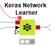
Once we define the network, we can train it and evaluate its performance. We train our network using the Keras Network Learner node:
This node requires the definition of:
- Input data, in our case images with shape 150x150 and 3 channels.
-
Target data, in this case the column with the 0-1 encoded classes.
-
Loss Function. For a binary classification task, we choose Binary Cross Entropy.
-
Epochs, batch size, and optimizer, in this case we train our network for 10 epochs with a batch size of 128 training data rows, and Adam as an optimizer. Additionally, we choose to shuffle training data before each epoch and set a random seed for reproducibility.
Tip: You can inspect the learning process by opening the Learning Monitor view as training progresses.
Next we apply our trained model to the test set. For that we rely on the Keras Network Executor node:

Here, we specify:
-
Input data, again in our case images with shape 150x150 and 3 channels. We set an input batch size of 32 testing data rows.
-
Output, where we define the converter that is used to transform the network output into table columns. In our case, we select “To Number (double)” since we want to inspect the values returned by the Sigmoid function.
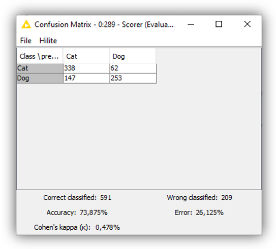
To evaluate the performance of our model, we first use the Rule Engine node to set a classification threshold and assign probabilities to one class or the other. For probability values ≥ 0.5 we assign the label “cat,” otherwise we assign the label “dog.” Second, we use the Scorer node to compute a confusion matrix and overall statistics (Fig. 10).
Finally, using the Keras Network Writer node, we export our trained model as an .h5 file for the deployment phase.
Note. The workflow Classifying Images of Cats and Dogs - Training is available for free on the KNIME Hub.
Deploy an Image Classifier
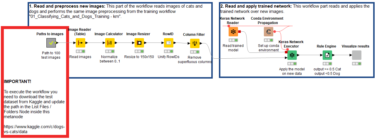
The deployment workflow mimics very closely the steps followed during training. After ingesting unseen image data, we normalize and resize it. Next, we import the trained model using the Keras Network Reader node and apply it using the Keras Network Executor node.
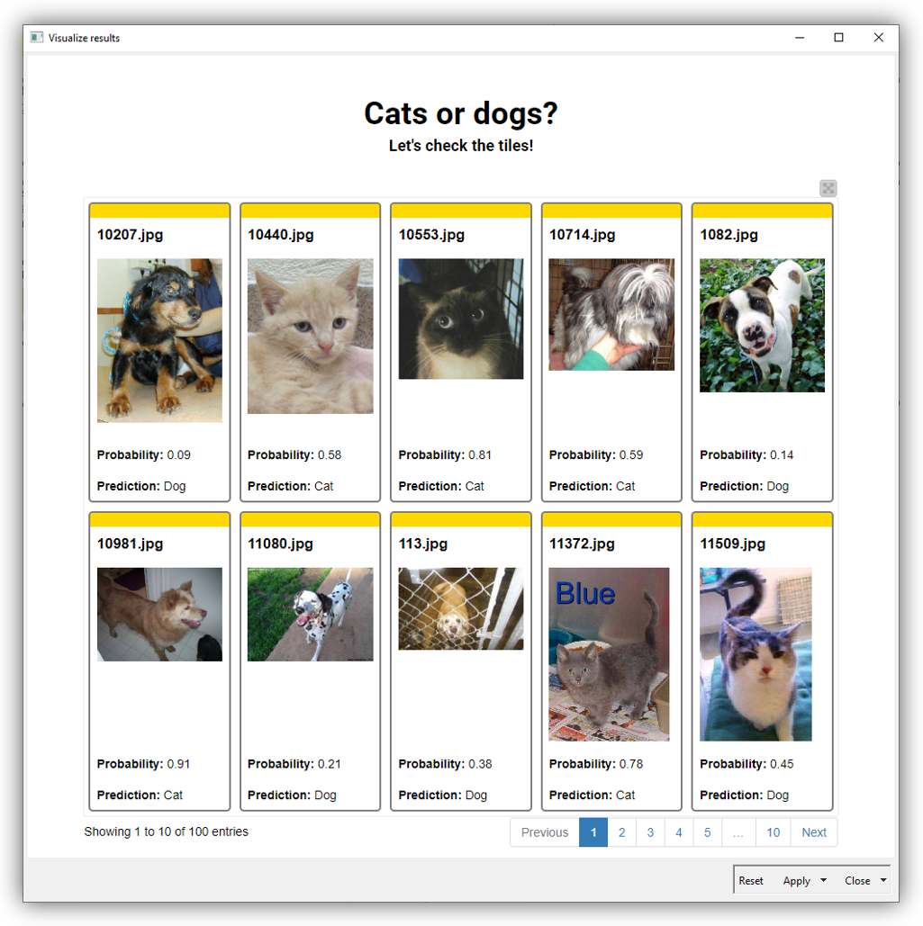
To assess the model performance on unlabelled data, we inspect the classification results visually. We build a simple dashboard using the Tile View node that displays the original image, the model prediction and probability (Fig. 12). We can see that in three cases the model fails to classify the input image correctly, but in two cases only by a small margin.
While satisfactory, the results suggest that performance improvements are possible and recommended. How? For example, we can add more Convolutional layers, optimize hyperparameters, ingest more training images, or use transfer learning.
Note. The workflow Classifying Images of Cats and Dogs - Deployment is available for free on the KNIME Hub.
Define Your Own Network For Freedom of Implementation
Image classification is a conceptually easy task, but for most tools, its implementation still requires overcoming the coding barrier.
KNIME’s Keras integration for deep learning allows us to define, train, and deploy deep neural networks in a fully codeless fashion. Combining a friendly GUI with visual programming, data teams can build complex workflows, drastically reducing implementation time, and also establish a strong human-machine interaction in which a data scientist can experiment quickly and transparently with different network topologies, architecture configurations, and hyperparameters for the creation of powerful AI solutions.