
Aging populations are causing the distribution of the data flowing into your model to drift. The upshot: Your income prediction model is no longer performing well. To help us monitor this prediction model, we can build an application that automatically throws an alarm when it detects data drift and retrains the model.
But to train this kind of model monitoring application and assess its performance, we need data that represent both the current and future conditions. Without a time machine, how can we get hold of future data?
We can generate synthetic data.
In this blog post, we want to walk through a workflow that enables you to synthetically generate (drifted) data for model monitoring. In a second article, we’ll describe how to build a model monitoring application.
Generating synthetic demographics data
We generate synthetic data to fast-forward and simulate a production environment years ahead and test whether the alarm triggers retraining of the model when needed. Future data can represent many different characteristics of the current customer data e.g., preferences and demographics of the current customers. But the drift might only affect one feature. In our example, the drift effects “age”.
The closest we can get to representing the drift is by generating synthetic data from the existing data.
In our synthetic data generation example, we are going to produce demographic data that shows older and older people, year by year, using the adult dataset as the current data. The adult dataset contains a sample of the census database from 1994, provided by the UCI Machine Learning Repository.
The prediction model we want to monitor could, for example, predict income class (below or above 50K per year). We also intend to apply the income prediction model in a production environment where “new adult data” is coming in daily, as one person per day.
And now here comes the data drift: The new person joining today was expected to be younger than the new person joining in five years. To get an idea, think about the population in western countries getting older and older every year. Consequently, the income prediction model would perform worse as time moves on from when the model was initially trained, because the deployment data gradually drifts further and further away from the training data.
The synthetic data we need in this case is, firstly, a larger sample of adult data to define the “normal”, and secondly, adult data with the statistical properties in five, six, seven, or more years to represent the drift.
Now let’s have a look at how to generate normal and drifted synthetic data in KNIME.
Introducing the data generation steps
We’ll generate the data by following the steps in the workflow below. If you want to refer to the workflow as we walk through this example, you can download it from the KNIME Hub.
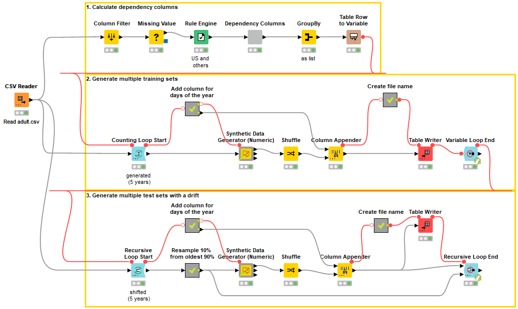
The workflow accesses the original adult dataset with the CSV Reader node. In part 1 (topmost yellow box), it calculates the interrelationships with the age column into which we are going to generate synthetic values. Next, in part 2, it generates the five training datasets that replicate the statistics and interrelationships in the original data. And finally, in part 3, it generates the test datasets that show the data drift.
Next, we’ll introduce these steps in detail.
Part 1: Calculating the interrelationships
Before generating the data into one column, in this case, the age column, we check for other columns that should be considered in the data generation to ensure, for example, that the average age is the lowest among the adults with a child at home.
We consider the interrelationships in the data generation by using different distribution parameters for different subsets of the data. In this case, we sample the synthetic values from a normal distribution, which is our (empirical) approximation of the distribution of the age values.
We use the Analysis of variance (ANOVA) test to find out the strongest interrelationships and thus the columns that should determine the subsets, as shown in the workflow below:
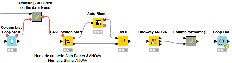
We start with the Column List Loop Start node to test the strength of the relationship with the age column for each column at a time. We then perform the ANOVA test for the equality of mean and variance of age between the groups in the current column with the One-way ANOVA node. For example, we test if the mean and variance of age are different between the groups “male” and “female” in the Sex column. For nominal columns, the groups are defined by unique values, such as “male” and “female”. For numeric columns, the groups are defined as five bins of equal frequency as created by the Auto-Binner node. Finally, inside the Column formatting metanode, we format the test statistics and their significance values and collect them for all columns with the Loop End node:
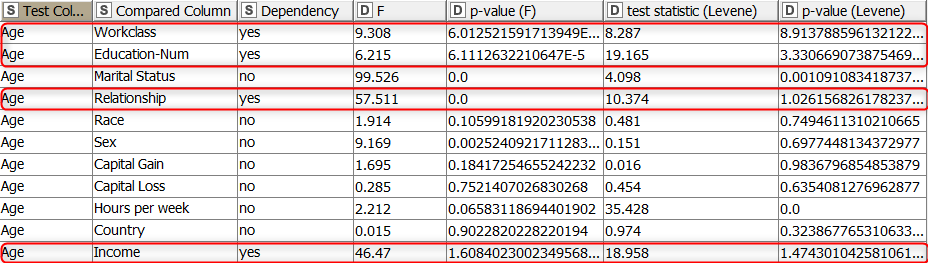
The output table shows for each column if it is related to the age column. The relationship is considered to exist if the p-values of the Levene test (equality of variances) and the F-test (equality of means) are below 0.001. In our example, the columns workclass, education, relationship, and income columns fulfill this criterion and are therefore considered when creating the sampling distributions of synthetic age values.
The next step is to generate data while considering these interrelationships.
Part 2: Generating synthetic data without a drift
We generate the training sets first. The training sets are adult datasets with random age values but with the same statistical properties as the original data. As shown in Figure 1, we start with the Counting Loop Start node to generate one training dataset per iteration. Within the loop body, we generate the age column with new, synthetic values with the Synthetic Data Generator (Numeric) component. After that, we randomize the row order in each dataset with the Shuffle node. This doesn’t affect the sample statistics but makes sure that the rows in each training set are not too similar. Finally, we write each dataset into a separate file with the Table Writer node. In our example we generate one data row for each day of the year, from 2020 to 2024.
The histograms in Figure 4 shows the distribution of the original (on the left) and generated (on the right) data:
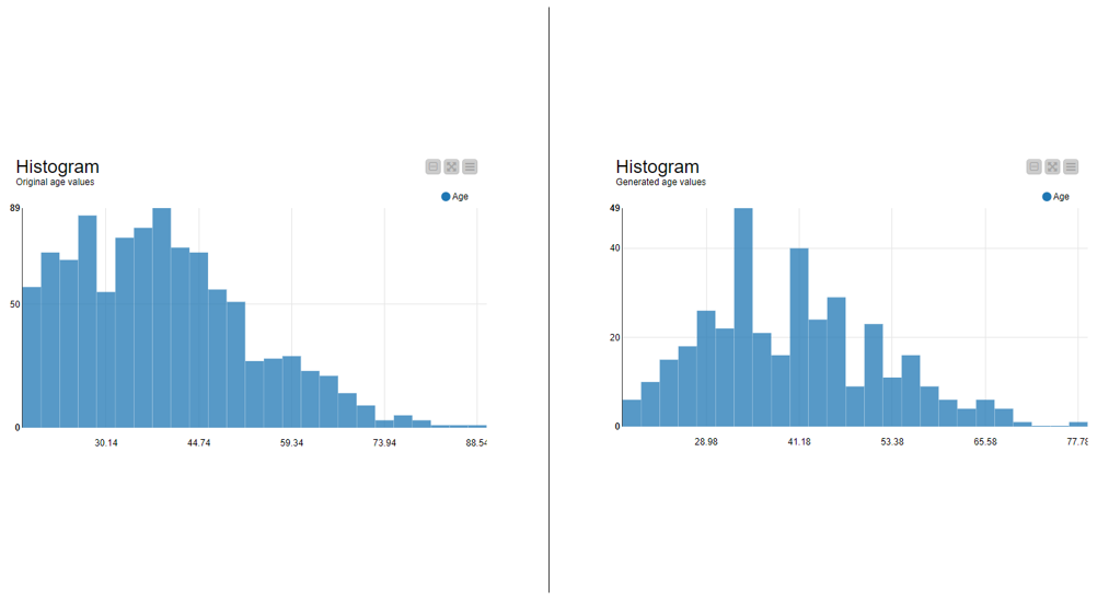
The original and generated age values have the same mean and variance as in the original subsets of the data. For example, the mean and variance of age is the same in the original and generated data in the group of unmarried people with less than 7 years of education working in the private sector and having income less than 50K per year. Since the data are generated from a distribution that only approximates the distribution of the original data, the generated data follows the normal distribution more closely than the original data.
Figure 5 shows the configuration of the Synthetic Data Generator (Numeric) component:
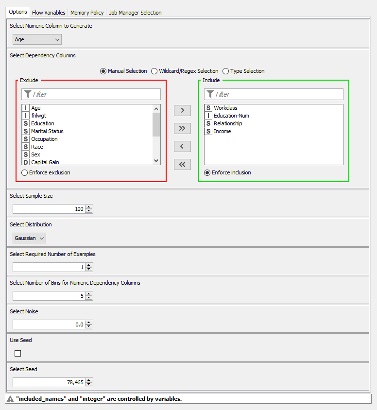
Starting from the top, we select the age column as the column to generate and relationship, education, income, and workclass as the dependency columns. We overwrite the sample size by a flow variable to correspond to the number of days (365 or 366) in the year. And lastly, we set the sampling distribution to Gaussian.
Further below in the configuration dialog, you can find additional settings such as the required size of a group and the fraction of noise in the generated data. With these settings, you could ensure that the original data cannot be reconstructed from the generated data and thus use the component for anonymization as well.
The top output of the component contains the generated age values, which is the only output we need here. The second and third output ports only show additional details of the sampling distributions.
Finally, we generate the test sets by introducing a drift into the original data.
Part 3: Generating synthetic data with a drift
In this final step, we generate test datasets where the distribution of age shifts to the right year by year. Furthermore, because a feature seldom shifts independently of the others, we consider the interrelationships here as well. Otherwise, if we only shifted the age column, we might end up with too many rows representing an unlikely scenario, for example, with people over 60 years having a child at home.
When we generate the test sets, the dataset for each year is supposed to contain older people than in the previous year. We take care of this by using a recursive loop (Figure 1) where we generate each new dataset based on the previous year’s dataset and replace the youngest 10% from the previous year’s sample with a random sample from the total population to introduce the drift. We do this inside the “Resample 10% from oldest 90%” metanode at the beginning of each iteration. Otherwise, the data generation steps are the same as for the training sets.
Furthermore, since the test sets should follow the training sets in the data pipeline, the “Days of the year” component generates timestamps that start from the year 2025 and end in 2029.
Figure 6 shows the generated training data (on the left) and the generated test data with a drift (on the right):
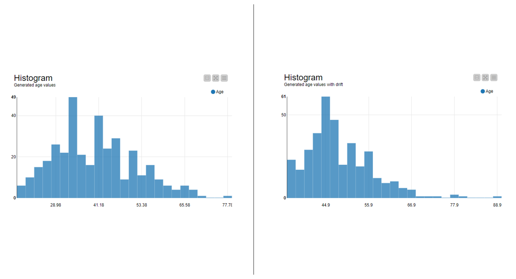
The distribution of the generated test data has a peak at about 44 years, whereas the generated training data has a peak at about 35 years. Furthermore, the left tail in the distribution of the training data is longer, because the training data contains a wider range of young age values than the test data. It’s the opposite for the right tail, where the training data shows age values only up to about 77 years, whereas the age values in the test data range up to 88 years.
With the five test sets we now have all the synthetic data we need to build a model monitoring application.
Looking Towards Model Monitoring
In this article, we’ve shown how to generate synthetic data with desired statistical properties and interrelationships to represent gradually drifting data in a production environment. We will use this synthetic data to test our model monitoring application.