
KNIME Analytics Platform is an open source tool that enables easy creation of workflows that can perform numerous kinds of data transformations in an intuitive way. The resulting workflows are not only easy to understand by people that have never seen the workflow, but also produce reproducible results.
In this blog post, we describe three KNIME workflows developed to work with near-infrared (NIR) spectroscopy data measured on chemical samples. NIR spectroscopy measures absorption (or transmittance) of light with wavelengths between 780 and 2500nm.
This method, which is non-intrusive and requires comparatively little sample preparation, is applied in a wide range of fields such as agriculture, product monitoring, polymer engineering, biomedicine, pharmaceutical industry, and environmental science. The method’s low sensitivity to minor experimental constituents makes it necessary to set up calibrations that require many samples. Additionally, raw data need to be preprocessed to account for the physical property of the sample particles such as particle size, density and scatter, before proceeding to quantitative analysis.
In this article we look at three workflows for the pre-treatment and analysis of NIR spectroscopy data.
- The first workflow, NIR Spectroscopy data pre-treatment, deals with data treatment and we look at how spectral data are preprocessed to compensate for the inherent conditions of NIR spectroscopy
- The second workflow, Visualization, Clustering, and PCA analysis of Preprocessed Spectral Data, produces visualizations, PCA, and hierarchical clustering of samples based on their corresponding spectral data
- The third workflow, Similarity Search Using Inhouse Database, demonstrates how to perform a similarity search for one or more spectra against a custom inhouse database.
1. NIR Spectroscopy data pre-treatment
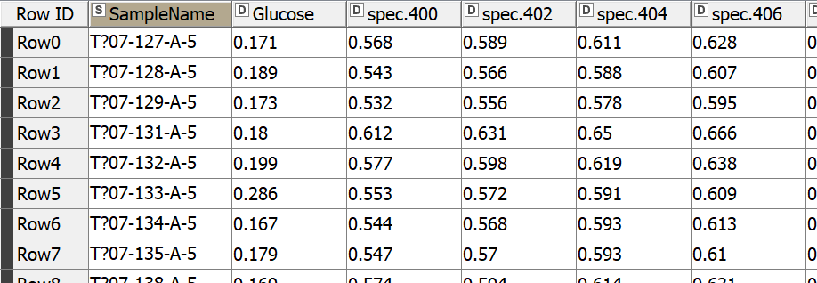
Let’s start by reading our NIR dataset, which is a challenge NIR spectra dataset obtained from https://github.com/mortenarendt/NIRchallenge/tree/master/Straw. The dataset is available as a matlab file and we used GNU Octave to convert it to a CSV format before reading it in KNIME Analytics Platform. The samples came from straws and are associated with the sugar potential of each straw. A straw’s value for energy production is highly tied to its sugar potential and is determined by a complex process with the help of an enzymatic kit. We took a subset of the dataset for the purpose of our blog post. In particular, we took 357 samples measured by NIR in the range 400-2498nm.
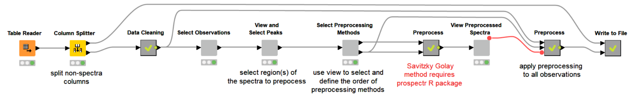
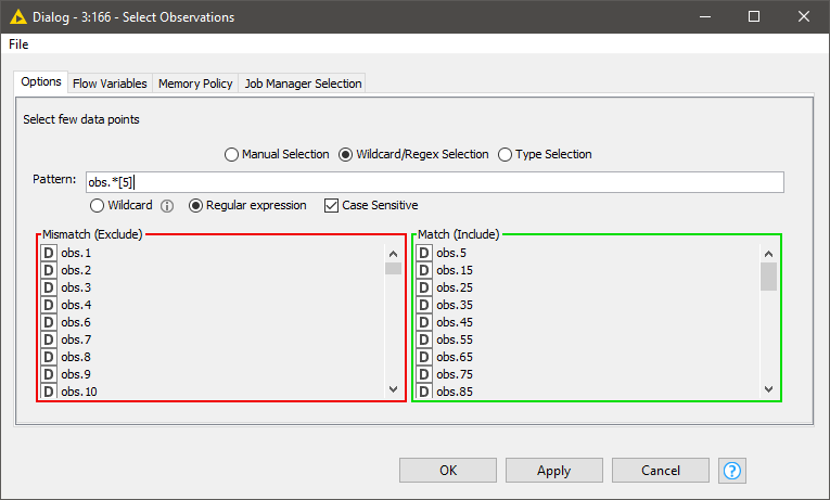
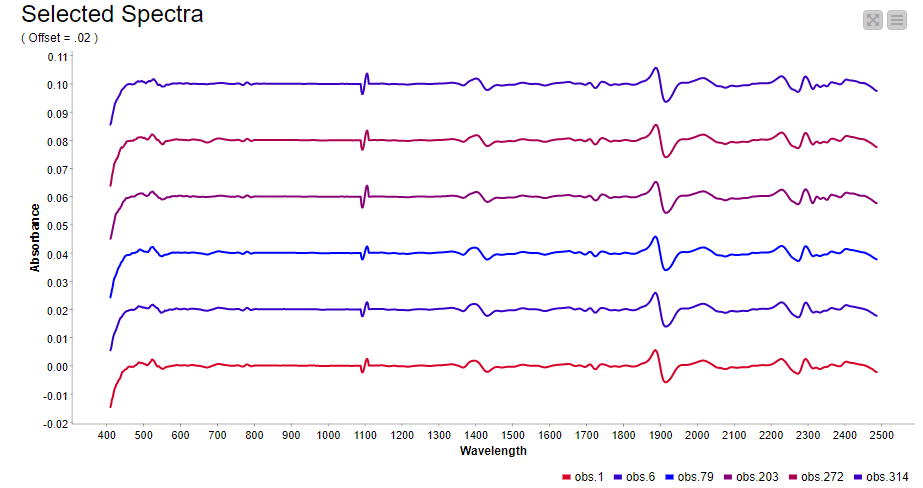
The first thing we want to do is visualize the spectra. Since it is difficult to plot and visualize the spectra of all 357 samples, we will select a few interactively. Doing this with a component with a column filter configuration is a good fit.
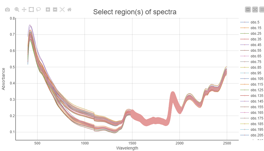
Once we have selected representative observations we can visualize their spectra and box-select the interesting regions that will be used for preprocessing. In this example we chose to use the region from 1500-2000nm for our preprocessing. The selection is highlighted as a thick line.
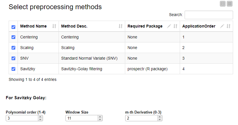
The next step is to decide which preprocessing methods to use and in what order they should be applied to the data.
In general, the most widely used preprocessing techniques can be classified into two categories. In the first category are the scatter-correction methods and in the second, the spectral derivatives. As representatives from the first category we selected Standard Normal Variate (SNV) and Normalization (Centering and Scaling) and for the second category Savitzky-Golay (SG) polynomial derivative filters 123.
Scatter correction methods are used to remove undesired spectral variations due to light scatter effects and variations in effective path length. SNV is a very simple method for normalizing spectra to correct for light scatter 1. It is calculated by subtracting the mean of spectrum from individual values and dividing the result by standard deviation of the spectrum. Normalization transforms the spectra matrix to a matrix with columns with zero mean (centering), unit variance (scaling) or both (auto–scaling). In contrast to SNV, which operates row-wise, normalization operates column-wise. The Savitzky Golay method fits a local polynomial regression on a signal using an equidistant width 2
The selection of preprocessing techniques is done using the interactive view of a dedicated component. Methods can be selected and their order can be defined by editing the table. If the Savitzky Golay method is selected, its three additional parameters (polynomial order, window size and m-th derivative) can be adjusted.
Now, if we execute and open the view of the last component, we can clearly see the effects of our selected preprocessing methods on the data.
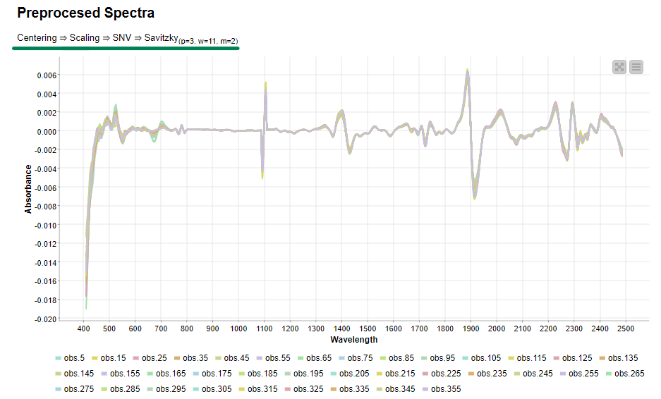
Once we verified that the preprocessing methods are working as expected, the same transformation will be applied to all samples to be preprocessed. Then we export the preprocessed data to disk for the next steps of spectral analysis
2. Visualization, Clustering, and PCA analysis of Preprocessed Spectral Data
Finding patterns in the data and deriving meaningful insights from this is among the strong features of the KNIME Analytics Platform. In our case this can be done through visualization, principal component analysis and hierarchical clustering. The second KNIME workflow makes use of the preprocessed data from above and does exactly these three things. We are still using the same dataset containing samples of straws associated with their sugar potential. The dataset was created to determine if NIR spectroscopy can be used to determine the sugar potential of straws instead of the complex process that involves enzymatic degradation.
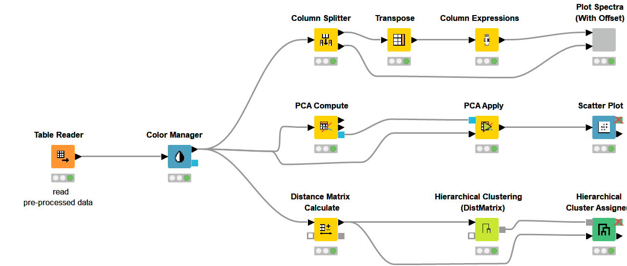
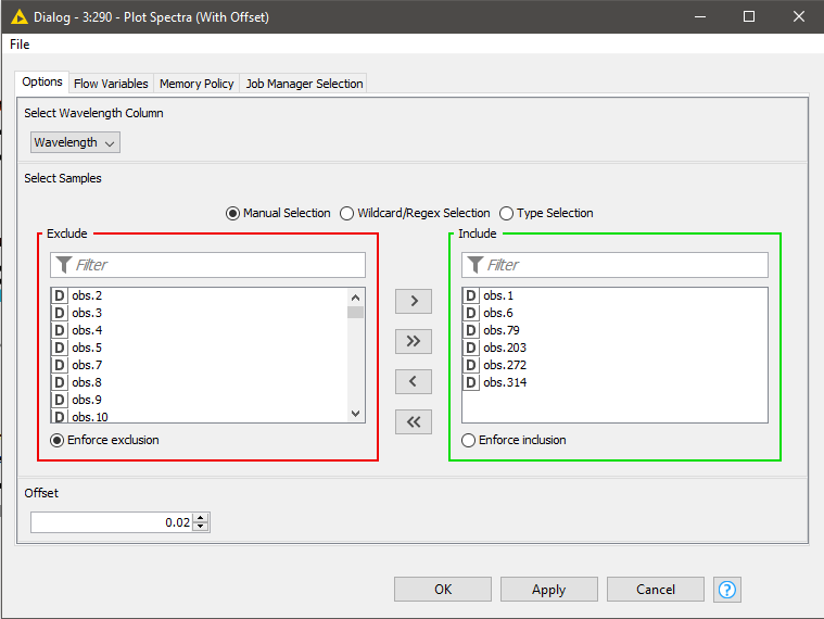
In spectroscopy, plotting multiple spectra as line plots for visual inspection of differences is a common task. To make the comparison easy, different spectrums are plotted with a fixed offset with the goal of avoiding overlapping lines. Using a configurable component (see component configuration dialog - Figure 9), where we can select the spectra to show in the plot and set the offset, plotting spectra can be done easily. The resulting plot is shown in Figure 9.
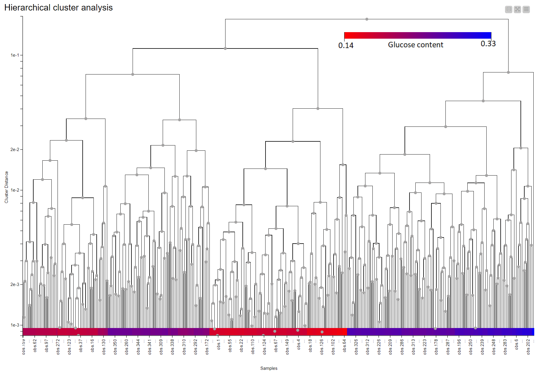
Hierarchical clustering in KNIME is simplified via the Distance Matrix Calculate node where we can compute the distance of choice between samples. Using a combination of just three nodes we were able to observe the clustering that is associated with the level of glucose in the straw samples. Samples are colored according to their glucose content measured by an enzymatic degradation and we can see that samples with similar glucose content tend to cluster together. This suggests NIR Spectroscopy has the potential to discriminate between good and bad straw samples (Figure 10).
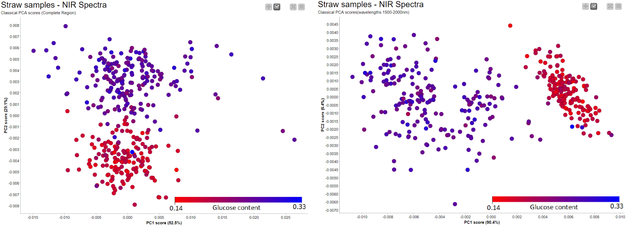
Similar to the Hierarchical clustering, PCA Analysis has the potential to reveal patterns and detect outliers. It can be performed easily using a couple of nodes in KNIME Analytics Platform. Figure 11 shows the results of a simple PCA analysis on the straw samples using the preprocessed spectral data. There is a clear separation between the straws with high potential for sugar (blue) and those with low levels of sugar (red). The PCA plot is the result of using the whole NIR range as input. We have a separation between samples, in terms of sugar level, across PC2 instead of PC1. This led us to think there is a more pronounced second pattern in the data which is unrelated to sugar level. When we went back to our preprocessing workflow and looked at where the samples show differences, we found two regions (700nm-1400nm and 1500nm-2000nm) with notable differences between the samples. After trying both regions, we picked wavelength region 1500nm - 2000nm and obtained the result on the right where we have a better clustering along the main principal component (PC1).
3. Similarity Search Using Inhouse Database
One of the applications of NIR spectroscopy is confirming the authenticity and quality of a chemical or food product by comparing it to a known reference product. At the heart of such applications is a method to measure the similarity between two spectra. Common methods in NIR spectroscopy are the correlation coefficient, the Euclidean, or the Mahalanobis distance. With this simple workflow, we will showcase how we can perform a database search of a spectrum using these (commonly used) distance measures.
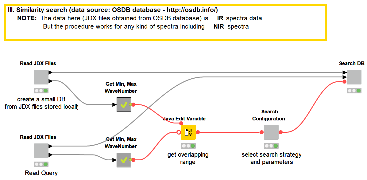
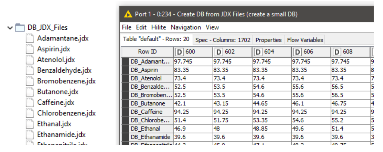
Storing spectral data in JCAMP-DX (.jdx) files is a common practice and many spectrometers directly produce data as .jdx files. We created a component that builds a spectral database by reading .jdx files contained in a folder, where each file represents a compound. After parsing individual .jdx files, the global wavelength ranges are detected and missing values (readings on a given wavelength that are present in compound A but not in compound B) are filled via linear interpolation. The result is a table where compounds are arranged row-wise and wavelengths in columns.
In this example, we are using 20 JDX files downloaded from http://osdb.info/ representing 20 different compounds to create our spectral database. The workflow can be adjusted to use a different list of JDX files with the goal of creating an own database. Figure 13 shows the list of compounds (files) that make up the database and the database itself shown as a KNIME table. This is a simple way of creating a database. For real world cases robust databases should be designed. For example, instead of a single spectral entry per compound, we can have multiple spectra representing multiple sources of variability associated with the product and the manufacturing process.
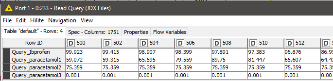
The next step is to read the query files that need to be searched against the database. We used a similar procedure as reading the database entries to read the queries as well. We have the spectra of Ibuprofen and three different readings of paracetamol (Figure 14).
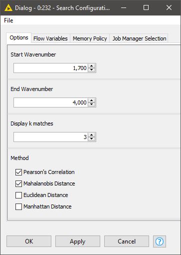
Once both the database and query tables are ready, we can define our search strategy via the configuration dialog of the Search Configuration component. This includes:
- The spectral region where the comparison should focus
- How many hits we should display per query
- Which similarity metrics to use
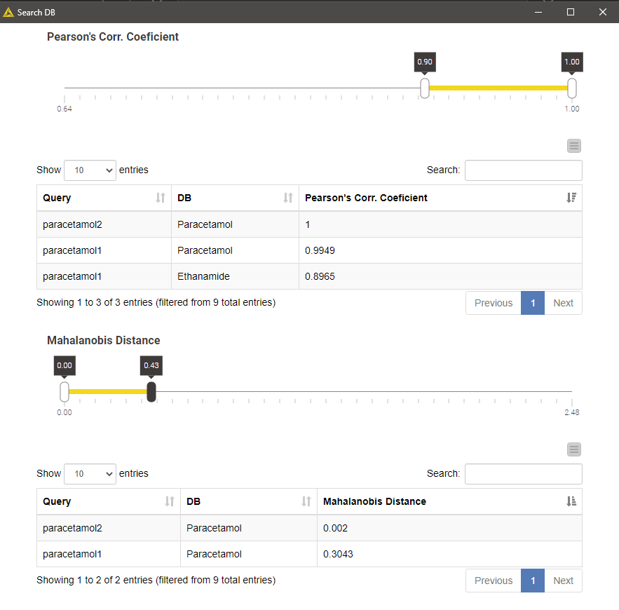
Executing the Search DB component and opening its view results in a list of top-k matches per query, or multiple lists if we selected more than one more than one similarity metrics. The list contains k matches irrespective of how good the matches are. We can filter the matches using the interactive range slider to enforce a certain degree of similarity index according to the search method in question.
The example result shown in the figure below is a result of searching two different paracetamol spectra against our tiny database using Pearson's correlation and Mahalanobis distance as similarity metrics. Not surprisingly, the database entry Paracetamol appeared as the best hit for both spectral queries and all search strategies.
Conclusion
We have shown three different KNIME workflows for NIR spectral data analysis. We have created a workflow that treats spectral data to account for experimental artifacts and method-related biases. Then we performed a PCA analysis and hierarchical clustering on the resulting data to determine if NIR methods can be used as an alternative way of measuring the sugar potential of straws. The results look promising as both our PCA analysis and hierarchical clustering results group straws with similar levels of sugar together. The PCA analysis also revealed the wavelength region 1500nm - 2000nm has a particular importance in relation to the sugar level of the straw samples. This is helpful information for further analysis such as creating a regression model that can actually predict the sugar potential of a straw from NIR spectral data. Finally we showed how an inhouse database can be created directly from jdx files and searched using different similarity search strategies with the aim of identifying a product or checking the authenticity of a product.
Taken together, we’ve demonstrated how KNIME Analytics Platform can be a powerful tool for typical spectra analyses. The workflows we provided can be downloaded from the KNIME hub and be adjusted to your own data.
References
1. Barnes, R. J., Dhanoa, M. S., & Lister, S. J. (1989). "Standard Normal Variate Transformation and De-Trending of Near-Infrared Diffuse Reflectance Spectra. Applied Spectroscopy", 43(5), 772–777
2. Abraham. Savitzky, M. Golay, (1964) "Smoothing and differentiation of data by simplified least squares procedures", Anal. Chem. 36 (8) 1627-1639 10.1021/ac60214a047
3. Stevens, Antoine, and Leonardo Ramirez-Lopez. "An introduction to the prospectr package", R Package Vignette, Report No.: R Package Version 0.1 3 (2014).