Word Embedding: Word2Vec Explained

This blog post is an extract from chapter 6 of the book “From Words to Wisdom. An Introduction to Text Mining with KNIME” by Vincenzo Tursi and Rosaria Silipo, which is published via KNIME Press.

Interpretability of the embedding space becomes secondary.

The Word2Vec technique is based on a feed-forward, fully connected architecture [1] [2] [3]. Let’s start with a simple sentence like “the quick brown fox jumped over the lazy dog” and let’s consider the context word by word. For example, the word “fox” is surrounded by a number of other words; that is its context. If we use a forward context of size 3, then the word “fox” depends on context “the quick brown”; the word “jumped” on context “quick brown fox”; and so on. If we use a backward context of size 3, the word “fox” depends on context “jumped over the”; the word “jumped” on context “over the lazy”; and so on. If we use a central context of size 3, “fox” context is “quick brown jumped”; “jumped” context is “brown fox over”; and so on. The most commonly used context type is a forward context.

Given a context and a word related to that context, we face two possible problems:

• from that context, predict the target word (Continuous Bag of Words or CBOW approach)
• from the target word, predict the context it came from (Skip-gram approach)

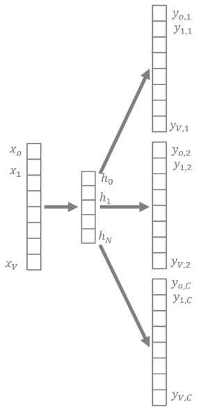
Let’s limit ourselves for now to context size C=1. If we use a fully connected neural network, with one hidden layer, we end up with an architecture like the one in Figure 1 for both approaches.

The input and the output patterns are one-hot encoded vectors, with dimension 1xV where V is the vocabulary size. In case of the CBOW strategy, the one-hot encoded context word feeds the input, and the one-hot encoded target word is predicted at the output layer. In case of the Skip-gram strategy, the one-hot encoded missing word feeds the input, while the output layer tries to reproduce the one-hot encoded one word context. The number of hidden neurons is N, with N < V.

In order to guarantee a probability based representation of the output word, a softmax activation function is used in the output layer and the following error function E is adopted during training:

where w_o is the output word and w_i is the input word. At the same time, to reduce computational effort, a linear activation function is used for the hidden neurons and the same weights are used to embed all inputs (CBOW) or all outputs (Skip-gram).

Figure 1. V-N-V neural architecture to predict a target word from a one word context (CBOW) or a one word context from a target word (Skip-gram). Softmax activation functions in the output layer guarantee a probability compatible representation. Linear activation functions for the hidden neurons simplify the training computations.

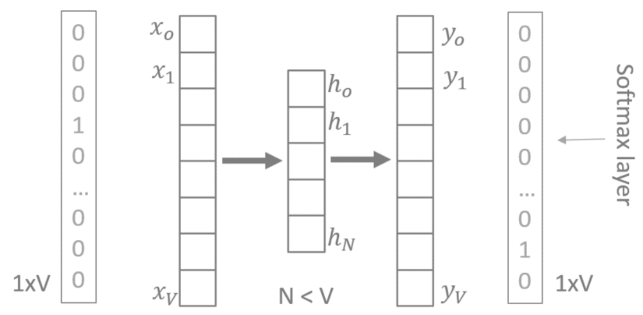
Notice that the input and output layers have both dimension 1xV, where V is the vocabulary size, since they both represent the one-hot encoding of a word. Notice also that the hidden layer has less units (N) than the input layer (V). So, if I represent the input word with the hidden neuron outputs rather than with the original one-hot encoding, I already reduce the size of the word vector, hopefully maintaining enough of the original information. The hidden neuron outputs provide the word embedding. This word representation, being much more compact than one-hot encoding, produces a much less sparse representation of the document space.

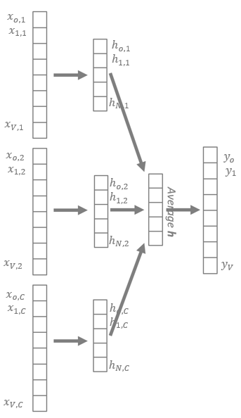
If we move to a bigger context, for example with size C=3, we need to slightly change the network structure. For the CBOW approach, we need C input layers of size V to collect C one-hot encoded word vectors. The corresponding hidden layer then provides C word embeddings, each one of size N. In order to summarize the C embeddings, an intermediate layer is added to calculate the average value of the C embeddings (Figure 2). The output layer tries to produce the one-hot encoded representation of the target word, with the same activation functions and the same error function as for the V-N-V network architecture in Figure 1.

A similar architecture (Figure 3) is created for the Skip-gram approach and context size C > 1. In this case, we use the weight matrix row, to represent the input word. Even here the word representation dimensionality gets reduced from V to N and the document space gets a more compact representation. This should help with upcoming machine learning algorithms, especially on large datasets and large vocabularies.

The vocabulary set can potentially become very large, with many words being used only a few times. Usually, a survival function examines all words in the vocabulary and decides which ones to keep. The survival function assumes the following form:

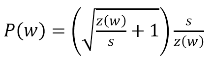
where w is the word, z(w) its frequency in the training set, and s is a parameter called sampling rate. The smaller the sampling rate, the less likely a word will be kept. Usually, this survival function is used together with a hard coded threshold, to remove very infrequent words.

Sometimes, in addition to the classic positive examples in the training set, negative examples are provided. Negative examples are wrong inputs for which no outputs can be determined. Practically, negative examples should produce a one-hot encoded vector of all 0s. The literature reports the usage of negative examples to help, even though a clear explanation of why has not been yet provided.

In general, the CBOW approach is already an improvement with respect to the calculation of a co-occurrence matrix, since it requires less memory. However, training times for the CBOW approach can be very long. The Skip-gram approach takes advantage of the negative sampling and allows for the semantic diversification of a word.

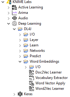
In KNIME Analytics Platform, there are a few nodes which deal with word embedding.

The Word2Vec Learner node encapsulates the Word2Vec Java library from the DL4J integration. It trains a neural network with one of the architectures described above, to implement a CBOW or a Skip-gram approach. The neural network model is made available at the node output port.

The Vocabulary Extractor node runs the network on all vocabulary words learned during training and outputs their embedding vectors.

Finally, the Word Vector Apply node tokenizes all words in a document and provides their embedding vector as generated by the Word2Vec neural network at its input port. The output is a data table where words are represented as sequences of numbers and documents are represented as sequences of words.

The whole intuition behind the Word2Vec approach consists of representing a word based on its context. This means that words appearing in similar contexts will be similarly embedded. This includes synonyms, opposites, and semantically equivalent concepts. In order to verify this intuition, we built a workflow, named 21_Word_Embedding_Distance and available on the KNIME Hub for you to download.

In this workflow we train a Word2Vec model on 300 scientific articles from PubMed. One set of articles has been extracted using the query “mouse cancer” and one set of articles using the query “human AIDS”.

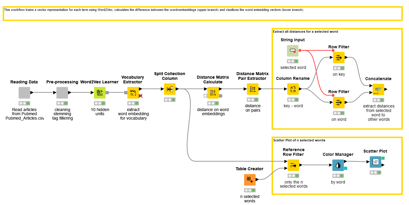
After reading the articles, transforming them into documents, and cleaning up the texts in the “Pre-processing” wrapped metanode, we train a Word2Vec model with the Word2Vec Learner node. Then we extract all words from the model dictionary and we expose their embedding vectors, with a Vocabulary Extractor node. Finally, we calculate the Euclidean distances among vector pairs in the embedding space.

Figure 4. EXAMPLES/08_Other_Analytics_Types/01_Text_Processing/21_Word_Embedding_Distance. You can download it from the KNIME Hub here. This workflow analyzes the embedding vectors of all words in the dictionary produced by a Word2Vec model trained on a dataset of Pubmed scientific articles. These Pubmed articles deal either with human AIDS or with mouse cancer. Distances between embedding vectors of word pairs are calculated.

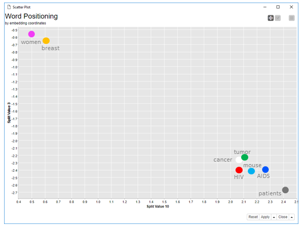
Figure 5 shows some results of this workflow, i.e. the positioning of some of the dictionary words in the embedding space using an interactive scatter plot. The interactive scatter plot allows for a drill down investigation across all pairs of embedding coordinates. For the screenshot below, we chose embedding coordinates #3 and #10.

In the embedding coordinate plot, “cancer” and “tumor” are very close, showing that they are often used as synonyms. Similarly “AIDS” and “HIV” are also very close, as it was to be expected. Notice that “mouse” is in between “AIDS”, “cancer”, “tumor”, and “HIV”. This is probably because most of the articles in the data set describe mice related findings for cancer and AIDS. The word “patients”, while still close to the diseases, is further away than the word “mouse”. Finally, “women” are on the opposite side of the plot, close to the word “breast”, which is also plausible. From this small plot and small dataset, the adoption of word embedding seems promising.

You can explore the embedding space using different embedding coordinates in the scatter plot. Just select the menu icon in the top right corner in the view window generated by the Scatter Plot (JavaScript) node and change the x- and y-axis.

Note. All disease related words are very close to each other, like for example “HIV” and “cancer”. Even if the words refer to different diseases and different concepts, like “HIV” and “cancer”, they are still the topic of most articles in the dataset. That is, from the point of view of semantic role, they could be considered equivalent and therefore end up close to each other in the embedding space.

Continuing to inspect the word pairs with smallest distance, we find that “condition” and “transition” as well as “approximately” and “determined” are the closest words. Similarly, unrelated words such as “sciences” and “populations”, “benefit” and “wide”, “repertoire” and “enrolled”, “rejection” and “reported”, “Cryptococcus” and “academy”, are located very closely in the embedding space.

Figure 5. Scatter plot of word embedding coordinates (coordinate #3 vs. coordinate #10). You can see that semantically related words are close to each other.

Displaying words on a scatter plot and analyzing their relations is just one of the many analytics tasks you can cover with text processing and text mining. From text cleaning to stemming, from topic detection to sentiment analysis, we have tried to describe the “how to” in the upcoming book.

This book extends the catalogue of KNIME Press books with a description of techniques to access, process, and analyze text documents using the KNIME Text Processing extension.

The book covers text data access, text preprocessing, stemming and lemmatization, enrichment via tagging, keyword extraction, word vectors representation, and finally topic detection and sentiment analysis.

For example, did you know that you can access pdf files or even epub Kindle files? Did you know that you can remove stop words from a dictionary list? Or stem Finnish words? Or build a word cloud of your preferred politician’s talk? Or build a graph of forum connections? Or use Latent Dirichlet Allocation for automatic topic detection? Or use the Word2Vec neural architecture to embed words?

• You will find all this and more in the book “From Words to Wisdom”.

[1] Le Q., Mikolov T. (2014) Distributed Representations of Sentences and Documents, Proceedings of the 31^st International Conference on Machine Learning, Beijing, China, 2014. JMLR: W&CP volume 32.

[2] Analytics Vidhya (2017), An Intuitive Understanding of Word Embeddings: From Count Vectors to Word2Vec

[3] McCormick, C. (2016, April 19). Word2Vec Tutorial - The Skip-Gram Model. Retrieved from http://www.mccormickml.com http://mccormickml.com/2016/04/19/word2vec-tutorial-the-skip-gram-model/