
In this blog series we experiment with the most interesting blends of data and tools. Whether it’s mixing traditional sources with modern data lakes, open-source devops on the cloud with protected internal legacy tools, SQL with noSQL, web-wisdom-of-the-crowd with in-house handwritten notes, or IoT sensor data with idle chatting, we’re curious to find out: will they blend? Want to find out what happens when IBM Watson meets Google News, Hadoop Hive meets Excel, R meets Python, or MS Word meets MongoDB?
Follow us here and send us your ideas for the next data blending challenge you’d like to see at willtheyblend@knime.com.
Today: SQL and NoSQL - KNIME meets OrientDB. Will They Blend?
The Challenge
Today’s challenge is to take some simple use cases – using ETL- to pull data from text files and place them in a database; extract and manipulate graph data, and visualize the results in OrientDB, the open source NoSQL database management system. We want to export table data from an SQLite database and a csv file and place them in a graph storage – mixing together SQL and NoSQL. Will they blend?
ESCO Dataset
Our dataset is ESCO data – the European Standard Classification of Occupations. ESCO is the multilingual classification of European Skills, Competences, Qualifications and Occupations. The information in this dataset is about different areas of the job market. ESCO classification identifies and categorizes skills, competences, qualifications and occupations. Similar occupations are combined into related sections defined by special codes. These codes form a taxonomy in which the leaves of the tree are occupations and branches refer to different job areas. As ESCO data also contain information about the skills that are necessary for the occupations, it seems pretty obvious that a good way to present this data as a graph!
OrientDB
We want to use OrientDB for graph data storage. It's a multi-model open source NoSQL database management system that combines the power of graphs with document, key/value, reactive, object-oriented, and geospatial models into a single scalable, high-performance operational database.
So why do we want to use OrientDB even though KNIME supports working with JDBC-compatible databases? The reason is that the concept behind the JDBC driver is not a good match when working with graphs; it’s not compatible with graph traversal. But as we want to use a graph to visualize our results after taking the data from an SQLite database and a csv file we needed a way to connect our data with OrientDB – which is a graph database.
In order to do so, we have developed five OrientDB nodes that use native OrientDB Java API:
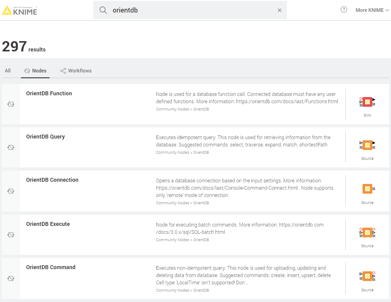
- OrientDB Function: The node is used for calling the server functions. OrientDB supports storing user-defined functions that can be written in SQL and JavaScript. It allows the user to execute some complex operations and queries without writing a script for it every time.
- OrientDB Query: Supports executing idempotent operations i.e. those that do not change data in the database. This way the node enables information to be extracted from the database. OrientDB has its own SQL dialect, which supports not only basic functions as any other SQL dialect, but also provides special graph traversal algorithms.
- OrientDB Connection: a node that allows you to create a connection to a remote or local OrientDB server. Here the user can specify the location and port of the database, its name, provide login and password, or use KNIME credentials. Once the connection is successfully created it can be propagated to other OrientDB
- OrientDB Execute: this node handles batch requests, this feature is very handy when you need to upload a large amount of data to the database. This way the user can specify the batch script or create it with the use of template.nodes.
- OrientDB Command: to enable executing non-idempotent operations i.e. those that can change data in the database. Consequently this node is used to insert, update, and delete data in the database. This node has 3 modes that make the work with it pretty flexible, we will discuss these modes further in the post.
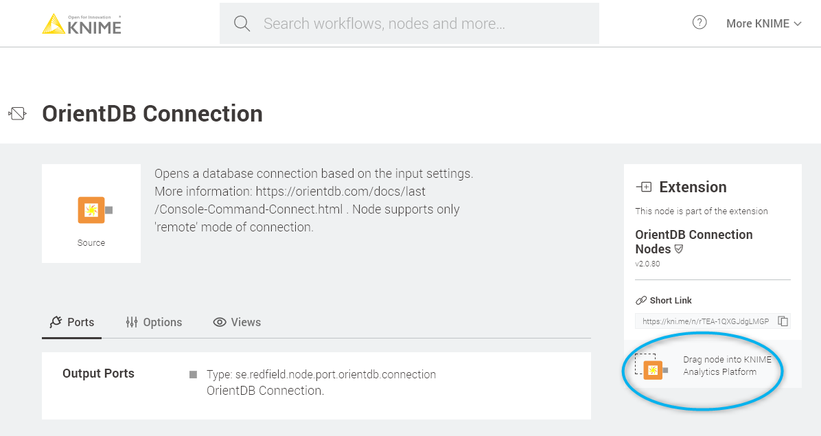
Tip: Look up the node you want on the KNIME Hub and then drag it into your workflow to start using it right away.
The Experiment
In our example, we use all these nodes and cover most of their modes and configurations in order to perform ETL from a relational database and a .csv file to graphs. We’ll also show you how you can export these data to KNIME and use network nodes for analysis and visualization.
Topic. Blending SQL and NoSQL; OrientDB integration with KNIME
Challenge. Perform ETL to OrientDB with KNIME, extract data from OrientDB and analyze it with KNIME
Access Mode / Integrated Extensions. OrientDB nodes, KNIME Network Mining Extension, JavaScript Views extension.
OrientDB is a very flexible database, organized based on graph schemas:
- Schema-Full: here you have a schema that defines the types of the classes and their properties
- Schema-Less: in this mode, the users can add as many new attributes as they want, on the fly
- Schema-Hybrid: here, both the above modes can be combined
It is also possible to use an OOP approach (Object-Oriented-Programming) in order to create different classes of vertices and edges.
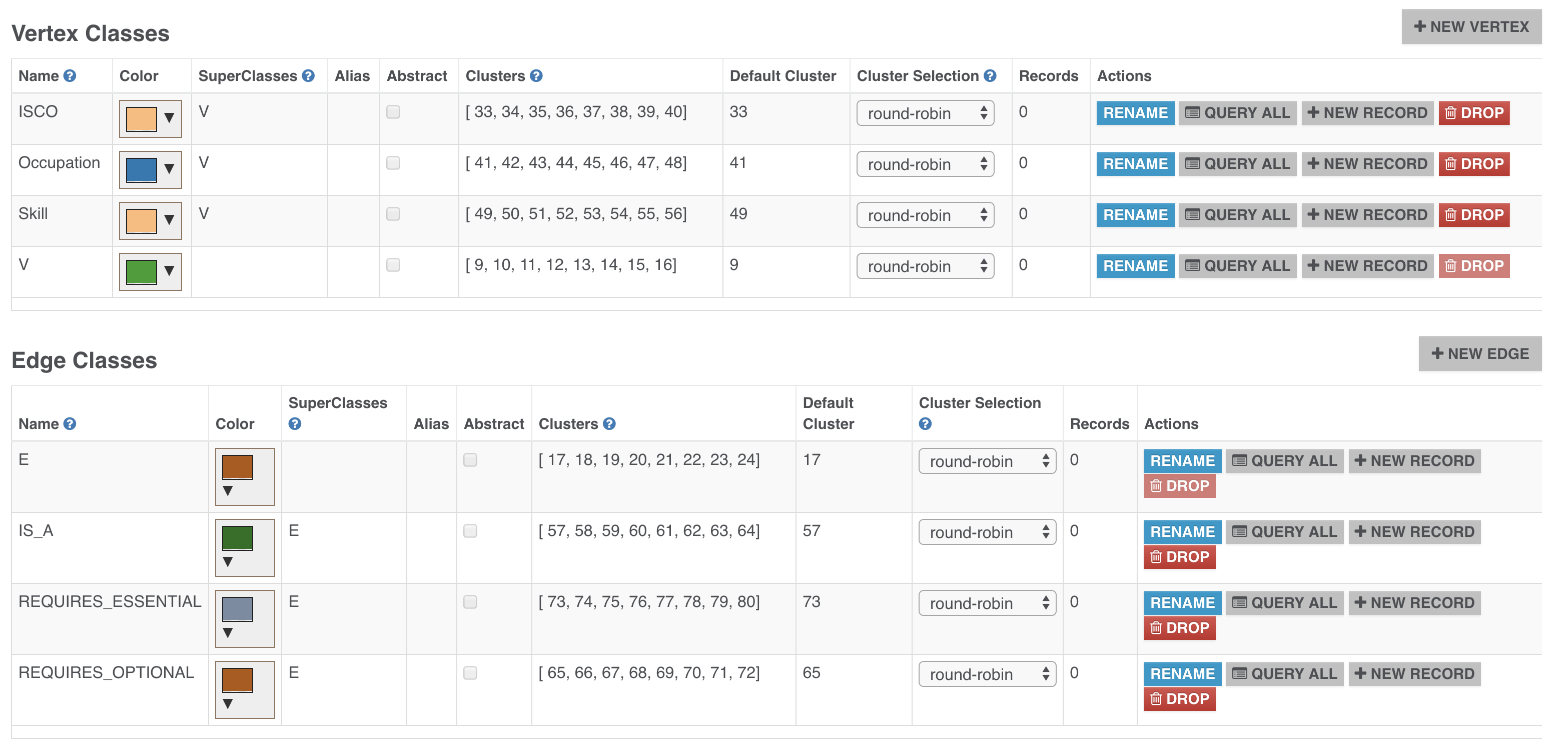
In this post, we are going to have three classes of vertices and four classes of edges that will be inherited from generic V and E classes for vertices and edges consequently. And, we will define a simple schema for these classes where all properties will be of String type.
Here is the script to create the schema:
We created the following vertex classes:
- ISCO (International Standard Classification of Occupations) class, which stands for ISCO code used for categorising occupations by different areas
- Occupation class, which defines a specific job in the ISCO classification system
- Skill class, which is used as the requirement for the occupation.
Now let’s talk about edge classes. We have the following:
- IS_A class, which is used to create ISCO taxonomy tree and connect it to the occupations
- Two REQUIRES_ESSENTIAL and REQUIRES_OPTIONAL edges to specify the skills necessary for the specific occupation
- SIMILAR_TO edge class, which will be used for defining similar occupations
Building the Workflow
Now that we have created a schema, we can start building the first workflow to fill the database. In this workflow (Figure 4) we read data from three tables stored in SQLite database – ISCO, Occupation and Skill, and one csv file that defines the skill requirements for the occupations. This workflow can be downloaded from:
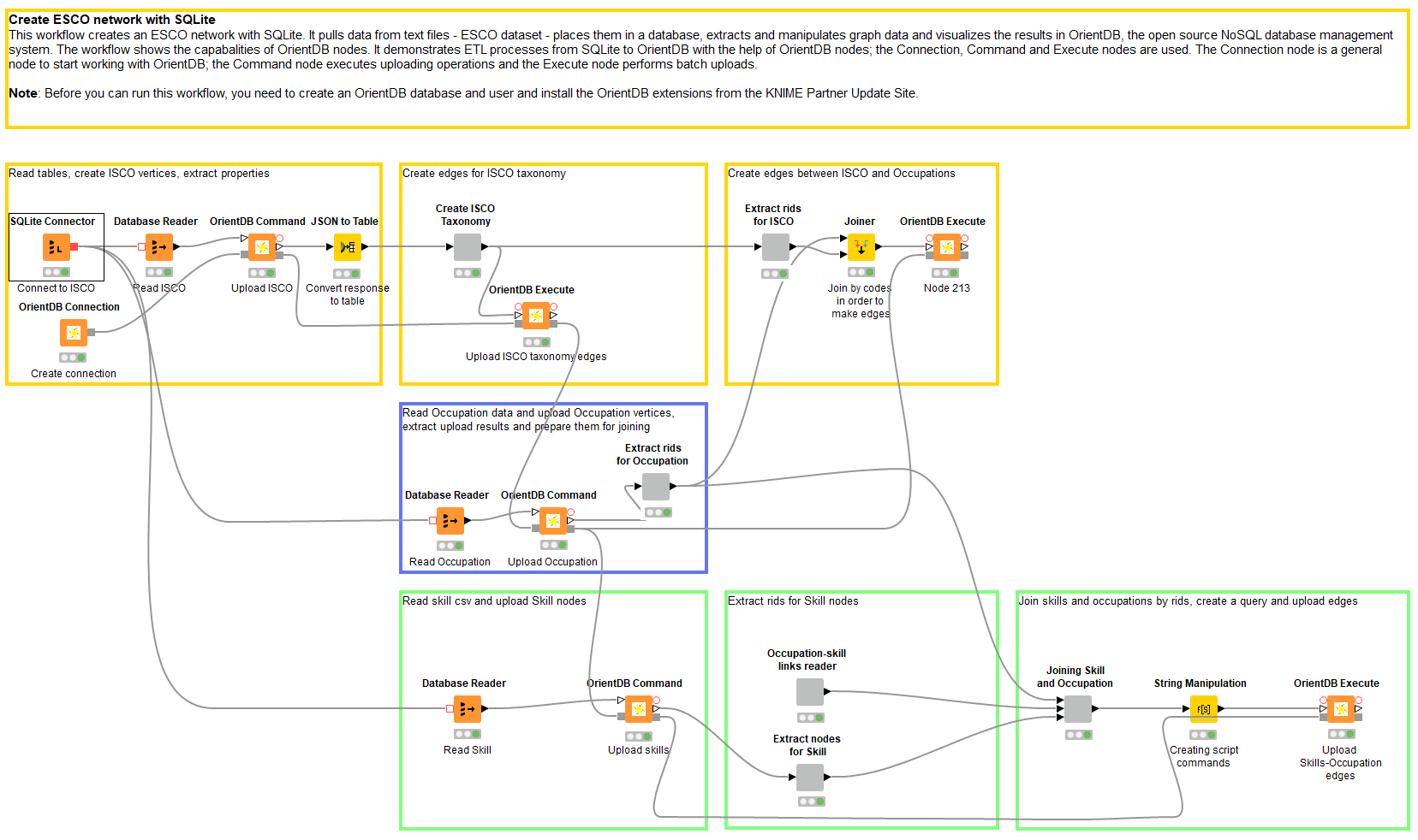
The SQLite database already contains the ISCO codes, occupations and skills, as a table. In order to analyze these data you need to extract all the tables into KNIME and do several expensive joins between these 3 tables. Obviously, these operations take a lot of time and computer resources, so as we are wanting to analyze the connections between several entities, it is more efficient to store such data as a graph. Reading data from an SQLite database is pretty straightforward; we used the Database Reader node. This node automatically returns data as a KNIME table. We can now propagate this table to the OrientDB nodes.
Once the data are read and put into KNIME tables, we can now connect and upload them into the database with the help of the Connection, Command, and Execute nodes. First we need to create the connection. The connection node settings are pretty simple (Figure 5).
You specify the following:
- Connection pool size
- Database URL
- Port
- Name
- There are two type of credentials: basic - login/password pair, and KNIME credentials, which can be created for the workflow.
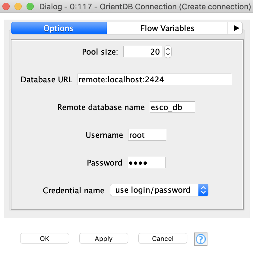
Once you have created the connection, it can be propagated to the other nodes.
Uploading ISCO codes
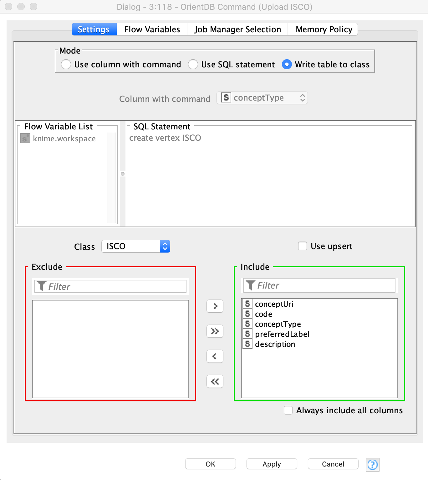
The next step will be to upload ISCO codes. For this task, we will use the Command node, which has three modes (Figure 6):
- «Use column with command» – here the user can provide a column that contains a string with queries that will be executed (execution goes row by row)
- «Use SQL statement» – in this mode the user can type the query into a text box. It is also possible to include flow variables in the query body
- «Write table to class» – here the user has to choose the vertex class that already exists in the database and then choose which columns will be uploaded to these class properties. Column names should be the same as the properties names in the class, otherwise new properties are created. This mode can also be used for updating information – to do this user has to activate the:
- «Use upsert» mode. This Upsert operation checks if the object with unique index already exists in the database. The included columns are used in the search, so the user does not have to specify certain columns. If the object exists, new values from selected columns are written. If the object does not exist, a new object is created.
Note: A good point about the Command node is that it returns the uploaded result as JSON. It is also fault-tolerant - this way if a record cannot be uploaded or updated for any reason, the user will have this message in the JSON output as well, without any runtime errors.
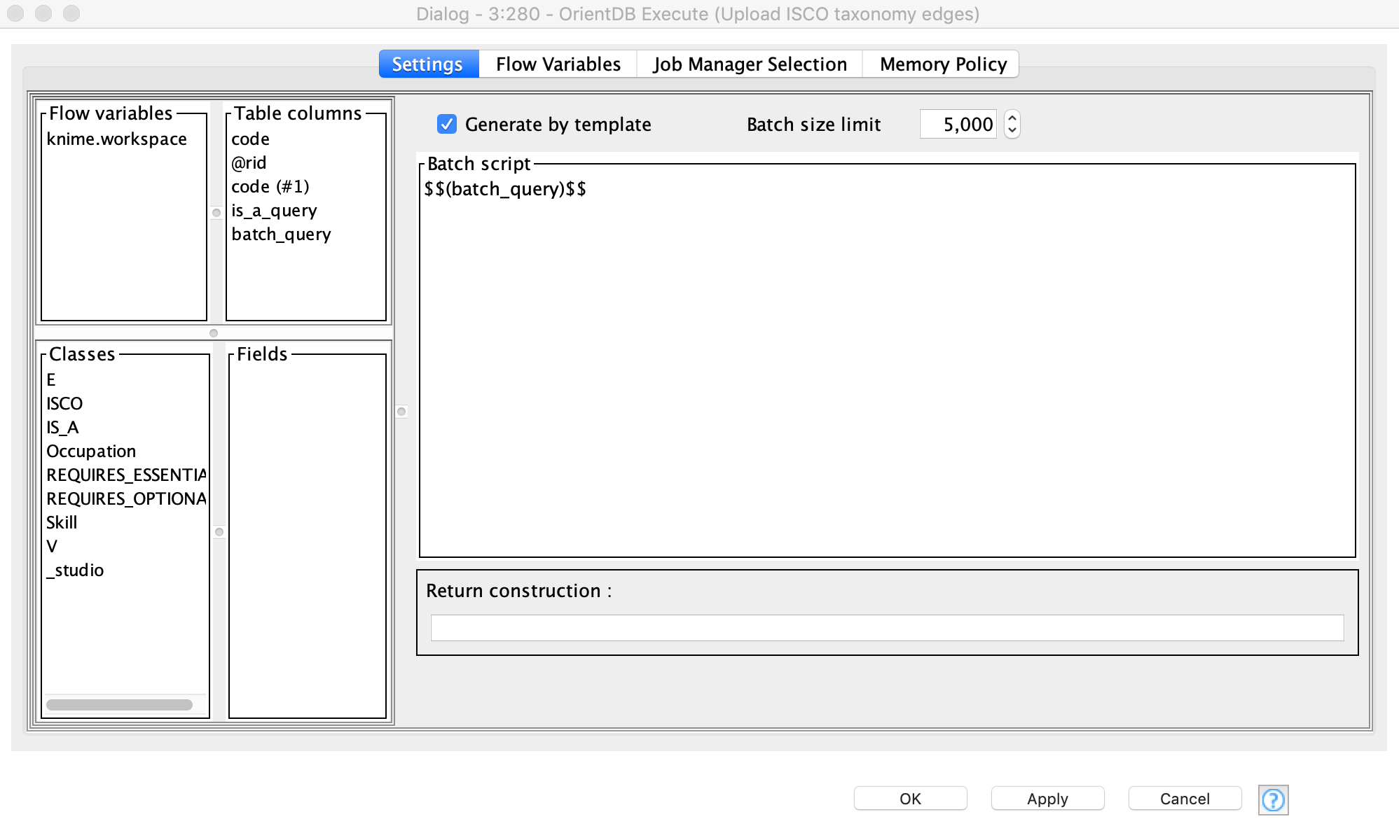
Now we want to use this JSON output and convert it to a KNIME table. After that, these data are used for creating edges. This way we can create a taxonomy of the ISCO codes, e.g. going from 0 to 01, to 011, to 0110. So once we have extracted the @rids of the created ISCO vertices (Figure 6), we create queries for edge-creation with the help of the String Manipulation node. The process of query-creation is performed in the «Create ISCO Taxonomy» component. This metanode has an output table, which contains a column with the queries that will be used in the Execute node (Figure 7).
Here we specify a name of the column with the query as the body of the script and activate the mode called «Generate by template» (Figure 8). This way the node automatically puts all the values from the selected column in to a script body. We use the default batch size here, as the script is not large, and we do not provide any return construction as we do not expect to get any results - our aim is to create edges.
We perform the same operations to upload the Occupation and Skill vertices:
- Read and preprocess the files;
- Use the Command node to upload them;
- Extract the output to get @rids in order to use them for other edge creation
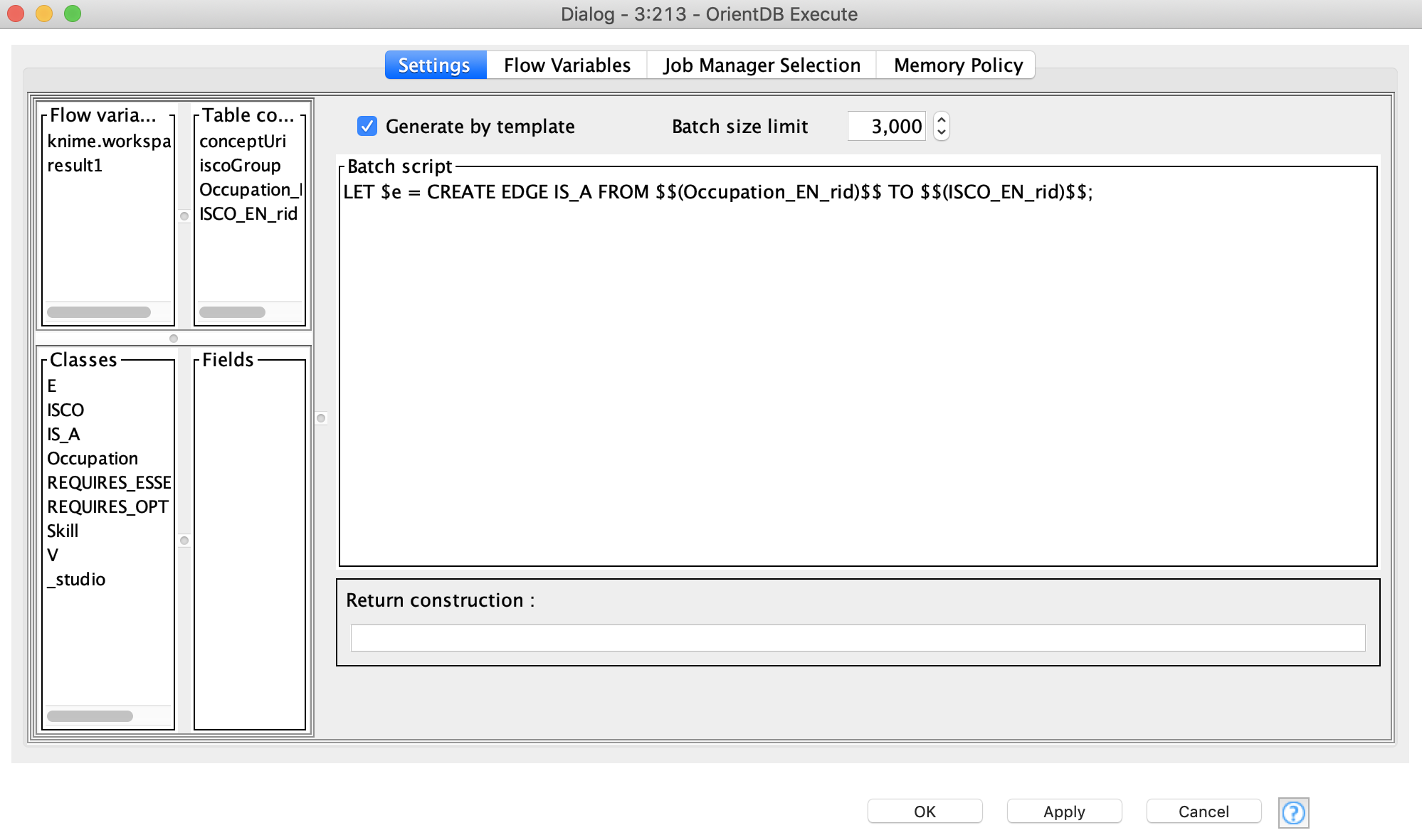
The next step is to create edges between the Occupation and ISCO vertices. The idea here is to join Occupation and the leaves of the ISCO vertices (these vertices have 4-digit ISCO code). Basically, Occupation should be connected to the last hierarchy level ISCO vertex. For this purpose, we join the ISCO table with the Occupation table by ISCO codes. We then use the Execute node again to create the edges, but in this case we create a template of the batch script in the text box, as shown in Figure 6. We put the similar string into a text box as we created for the previous Execute node, but also use columns as the wildcards for Occupation @rid values and ISCO @rid values.
In order to create edges between the Occupation vertices and the Skill vertices we need to read an additional table. The «Occupation-skill links reader» component takes care of this. This file also contains information about whether the skill is essential or optional for a specific job.
Joining
Now, we need to join this table with the results of the Command nodes, so as to upload the Occupation and Skill vertices. We join conceptUri with skillUri and occupationUri. These two joins are pretty expensive operations; fortunately we only need to do them once. After that, we create a script template again with the help of the String Manipulation node and propagate it to the Execute node.
That was the first part of the post – ETL. Now let’s consider some use cases for how these data can be extracted from OrientDB and used for analysis with some KNIME extensions.
Extracting Data from OrientDB and Analyzing with KNIME
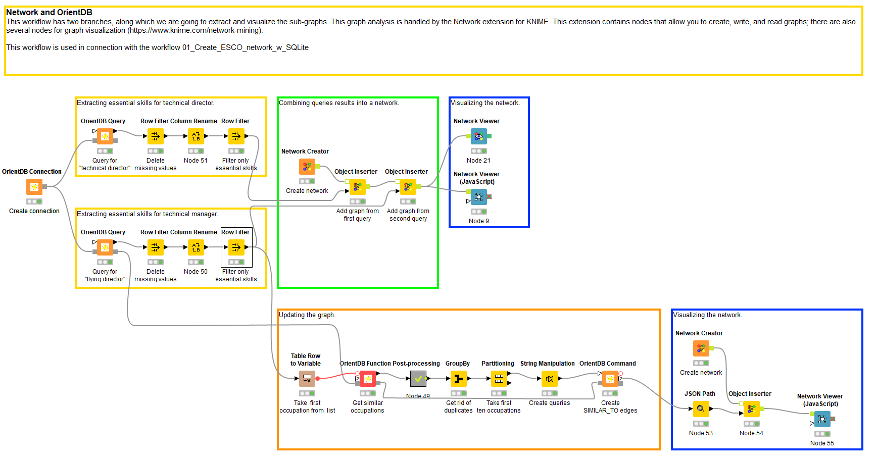
This workflow has two branches, along which we are going to extract and visualize the sub-graphs. This graph analysis is handled by the KNIME Network Mining Extension. This extension contains nodes that allow you to create, write, and read graphs; there are also several nodes for graph visualization (https://www.knime.com/network-mining). See Figure 9 where these parts of the workflow are enclosed in blue boxes.
First, we connect to the same database with Connection node.
Next, we create two independent queries to search for those skills essentially required for «technical director» and «flying director», see Figure 10. To run these queries we use the Query node.
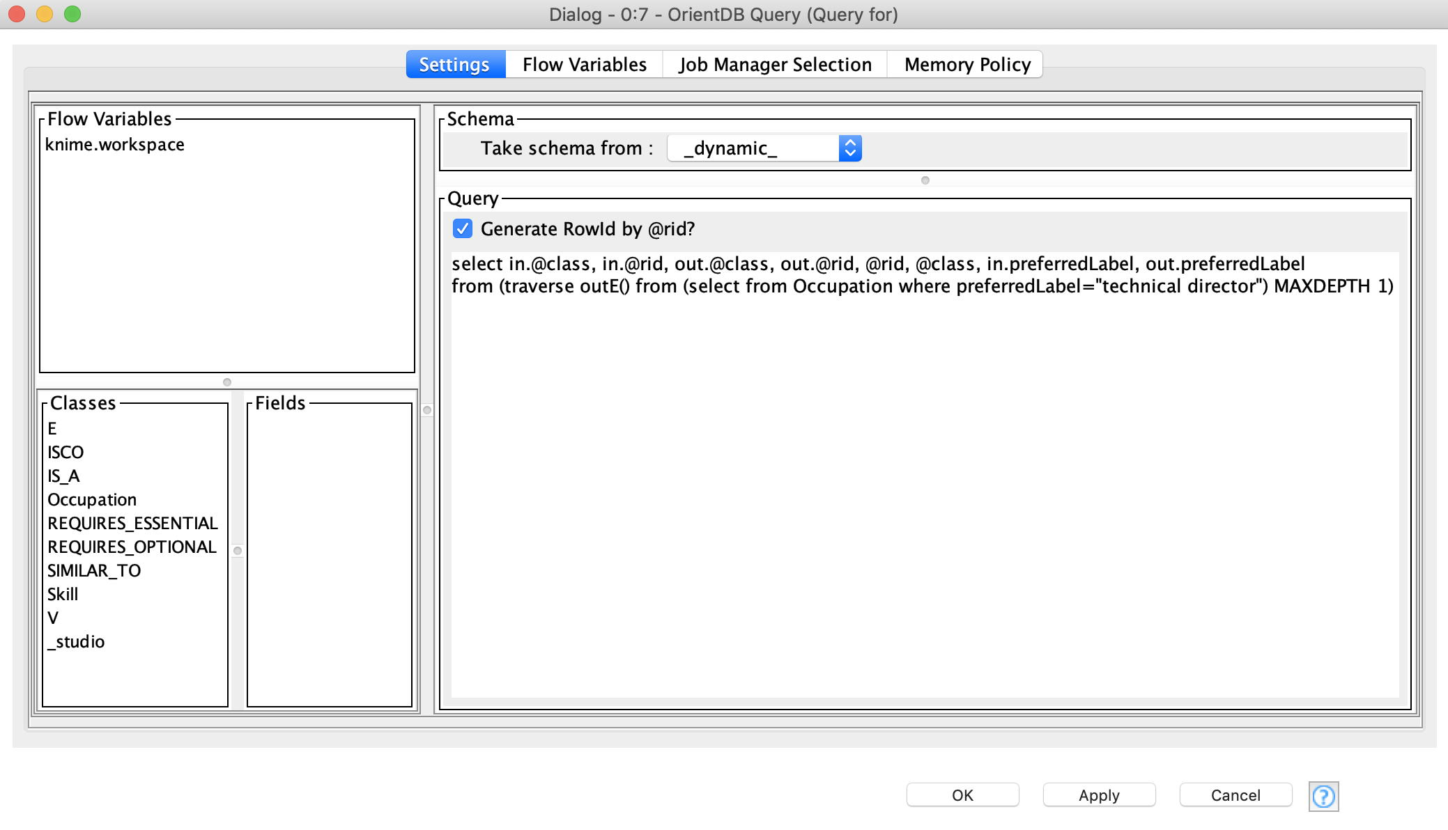
Configuring this node is similar to the settings in the Command and Execute nodes. The Connection node can automatically fetch metadata from the database: classes and their properties. The user could use these metadata and flow variables as wildcards in the query.
TIP: Choose the schema type depending on the result of the query. There are three main modes:
- Dynamic schema - general schema mode, which creates an output table according to the query results
- Class schema - returns a table according to the selected class
- JSON - returns the result as a table with JSON values
Since we want to extract information from different classes and specify which columns should be included in the result, we are going to use dynamic schema mode.
Preparing Extracted Data for Visualization
In order to prepare the extracted data for visualization, we need to create a network context with the Network Creator. No settings are needed for this node, we can simply start adding extracted and processed query results, i.e. the skills essential for the selected occupations.
We can now put them into the network we created, using the Object Inserter nodes. In the settings we need to specify IDs and labels for the nodes and edges. As you can see we extracted the data from the database in pairwise format, so we can specify the start and end vertices, and the edge type that connects them in the settings of Object Inserter, see Figure 11.
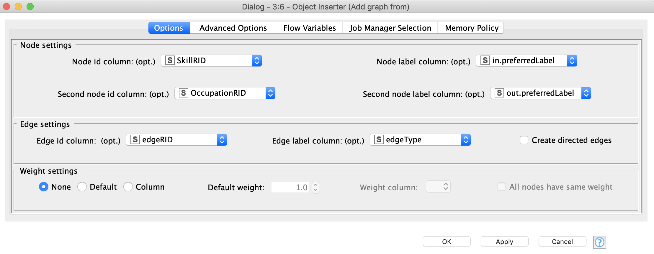
To add the result of the second query, all you need to do is propagate the network to another Object Inserter node and provide it with the table from the second query.
Network Visualizations
There are two nodes you can use for network visualizations:
The most important settings in these nodes are the layouts and label setup. Both nodes provide a Plot View with interactive elements, meaning you can change the visualization parameters on the fly, and after that generate an image in PNG and SVG formats.
OrientDB Function Node
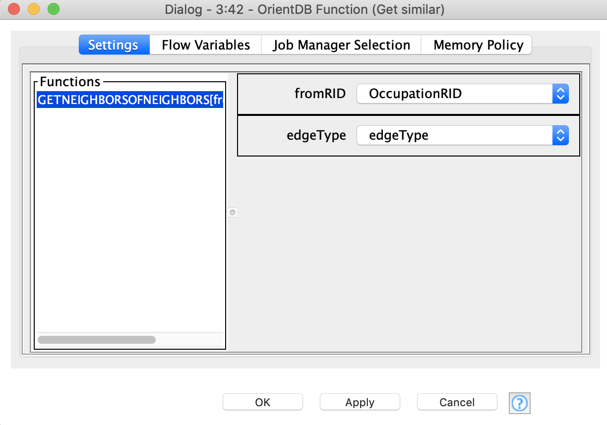
The lower branch of the workflow takes the first record from the second query («flying director» skills) and with the help of a server-defined function, returns all those occupations that require the same skills as «flying director». The functions can be written in SQL or JavaScript. We are going to use the following JS function:
This function has two arguments – the @rid of the start vertex and the type of the edge that is used for traversal. The Function node automatically fetches the list of functions that are defined by the user in the database. Once the user has selected the function, the arguments must be provided. This can be done in two ways – by using wildcards from the table columns or flow variables. In the first case the function is called for every record in the column, in the second case just once, see Figure 10.
The node returns the result as a JSON table since it is impossible to predict the output structure. This way, we need to convert it into a KNIME table, post-process and get rid of the duplicate @rids. After that, we take just the first 10 records from the top, and create for each of them the query to create an edge of SIMILAR_TO class to connect to the original «flying director» vertex. Next, we visualize the result in another network instance (Figure 13).
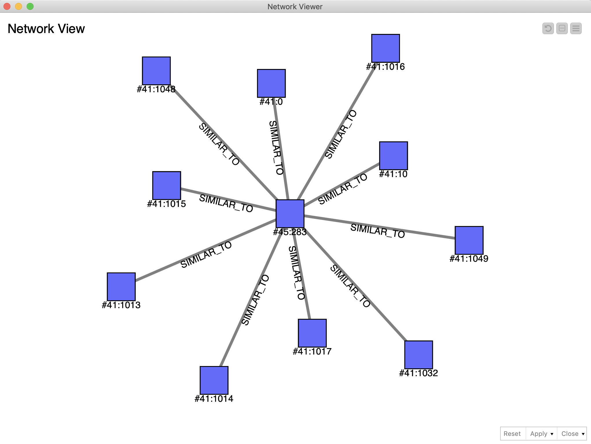
The Results
In this experiment we wanted to see if we could blend SQL and NoSQL in a workflow so as to be able to extract and manipulate graph data based in an OrientDB database. We used our OrientDB nodes to be able to do this, making it very easy to blend KNIME capabilities for ETL, data analysis, and visualization, utilizing the power of graph data representation, provided by OrientDB.
One of the benefits of using a graph as a storage is that many search operations can be reduced to searching a path i.e. a graph traversal. In the second part of the blog post we considered the use case of finding occupations that require similar skills. Using SQLite or any other relational database, this operation would usually require at least three joins. And these join operations would be required every single time we carried out such a search. By moving to a graph-based database, all of this information is already stored as edges. This approach saves a lot of time.
So yes, we were able to blend SQL and NoSQL and KNIME met OrientDB!
Future Work
Graph data representation provides huge benefits areas such as crime investigation and fraud analysis, social network analysis, life science applications, logistics, and many more. We plan to write more posts about integrating KNIME and OrientDB and reviewing other interesting use cases. Furthermore we continue to work on developing the OrientDB nodes in KNIME, so new features will be reviewed in the future articles.
References
- Summary of Redfield's OrientDB nodes on GitHub
- Links to these example workflows on the KNIME Hub
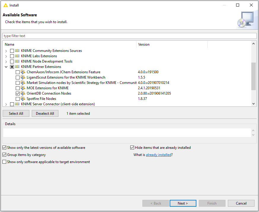
- How to Install the OrientDB nodes
- Go to the File menu in KNIME Analytics Platform 4.0 and select Install KNIME Extensions
- In the dialog that appears, expand KNIME Partner Extensions and select OrientDB Connection Nodes
------------------------------------
About Redfield
Redfield is a KNIME Trusted Partner. The company is fully focused on providing advanced analytics and business intelligence since 2003. We implement KNIME Analytics Platform for our clients and provide training, planning, development, and guidance within this framework. Our technical expertise, advanced processes, and strong commitment enable our customers to achieve acute data-driven insights via superior business intelligence, machine and deep learning. We are based in Stockholm, Sweden.