Stuck in the Nine Circles of Hell? Try Parameter Optimization & A Cup of Tea

Every data scientist has been there: a new data set and you’re going through nine circles of hell trying to build the best possible model. Which machine learning method will work best this time? What values should be used for the hyperparameters? Which features would best describe the data set? Which combination of all of these would lead to the best model? There is no single right answer to these questions because, as we know, it’s impossible to know a priori which method or features will perform best for any given data set. And that is where parameter optimization comes in.

Parameter optimization is an iterative search for the set of hyperparameters of a machine learning method that leads to the most successful model based on a user-defined optimization function.

Here, we introduce an advanced parameter optimization workflow that uses four common machine learning methods, individually optimizes their hyperparameters, and picks the best combination for the user. In the current implementation the choice of features and one hyperparameter per method are optimized. However, we encourage you to use this workflow as a starting point or a template if you have completely different data and customize it by including additional parameters into the optimization loop (and we will show where you could do that).

The parameter optimization workflow is shown in Figure 1 and is available on the KNIME EXAMPLES Server.

• Download the Model Optimization and Selection workflow from the KNIME Hub here

Figure 1. Overview of the parameter optimization workflow. Optimization for each candidate machine learning method is encapsulated within the corresponding metanodes.

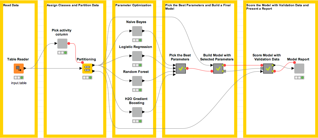
The workflow starts by reading in a data set. For this blogpost, we compiled a subset of 844 compounds, i.e. molecules, from a public data set available via https://chembl.gitbook.io/chembl-ntd/. This is a typical bioactivity data set where compounds have been tested for activity against a particular biological target, in this case CDPK1. Finding compounds that are active against a biological target is important for finding cures for the disease that is associated with this target. In our case, this target controls several stages in the life cycle of a malaria parasite and is therefore an attractive target for drug discovery research.

The compiled data set has two classes: 181 compounds interacting with the target have been assigned to the “active” class, the remaining 663 compounds are tagged “inactive”. Compounds are represented as molecular structure images and in order to obtain their numeric representations for machine learning we used a fingerprinting technique. We computed five chemical fingerprints for the compounds using the RDKit nodes in KNIME Analytics Platform and provided them with the data set. Since this blogpost is devoted to the topic of parameter optimization, we’ll leave out data preprocessing details.

In the next step of the workflow, the user selects a column containing class values in the Pick Activity Column Wrapped Metanode (by default the column “activity” is used). This column is used to perform random stratified partitioning of the data into a training set for parameter optimization and a test set for scoring the best model. The training data flows into one of the gray Wrapped Metanodes that carry the name of a machine learning method. Inside each of these nodes a parameter optimization loop is implemented. Once the optimization part is finished, the parameters and the performance statistics for the best model are extracted through a series of Metanodes. These parameters are used to train the final model. The last but not least piece of this workflow presents the scoring results to the user via the Model Report Wrapped Metanode.

Let’s dive into the parameter optimization step that’s being carried out inside the Wrapped Metanode for each method. We use Wrapped Metanodes here in order to encapsulate complex data processing and numerous flow variables. Let’s look at this in more detail in the Random Forest Wrapped Metanode (Ctrl/Cmd and double click the node to open it).

Figure 2. Parameter optimization sub-workflow for the Random Forest machine learning method.

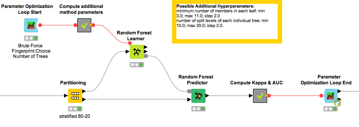
The sub-workflow we see inside the Wrapped Metanode is built on a standard parameter optimization workflow available on the KNIME EXAMPLES Server. If you want to know more about optimization loops, here is a related YouTube video “Parameter Optimization Loop”. We define the hyperparameters to be optimized in the configuration settings of the Parameter Optimization Loop Start node.

Figure 3. Configuration settings of the Parameter Optimization Loop Start node.

In the current implementation of the parameter optimization for the Random Forest model, we try optimizing the following parameters to get the best classification performance:

1. The fingerprint type (param_FPs);
2. The minimum size of the leaf (min_leaf_size);
3. The tree depth (tree_depth);
4. The optimal number of trees in the forest (forest_size).

For each one of these parameters, the start and stop values, as well as the step size, are defined inside the Configuration dialog of the node. We are using the BruteForce search strategy, which explores all possible combinations of the parameter values and picks the best one.

Notice that two parameters inside the Configuration dialog have the same start and end point, which means that they do not change their values during the optimization process. We’ve done this to make the demo workflows run faster; however, these parameters could also be optimized and we encourage readers to try this out in order to find the implementation of the parameter optimization for Random Forest that works best for them. With this in mind, we list additional hyperparameters along with their possible value ranges in the yellow-framed annotation boxes.

One should keep in mind that inside the parameter optimization loop for each machine learning method the data is partitioned once again. We use the same random seed across the four methods to ensure that the optimization is applied to the same partition of the training set and we can directly compare the results of the different methods.

The optimized parameters are used to build a final Random Forest, predictions are generated for the held-out validation data, and statistics are generated inside the Compute Kappa & AUC Metanode and passed to the Parameter Optimization Loop End node.

Figure 4. Configuration dialog of Parameter Optimization Loop End node. Here we optimize the paramters by maximizing the value in the flow variable named “Enrichment factor at 5%”.

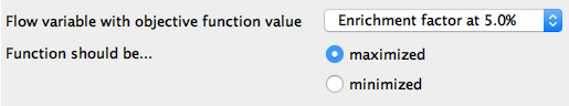
In the Configuration window of the Parameter Optimization Loop End node we select the optimization criterion used to determine the best parameter values for the model. Since the data set has an uneven class distribution and we plan to use the model to rank future compounds, we choose Enrichment factor at 5% (EF5) as the criterion. EF5 is defined as the ratio of the number of correct picks in the first 5% to the number we'd expect to get by picking randomly. There are, of course, other criteria that can be used to score a model, so the user can select different performance parameters, such as overall model accuracy.

We have now found the parameters leading to the best Random Forest model. You could imagine finishing the exercise here. However, we are interested in finding the best model across four machine learning methods, so we perform an analogous parameter optimization inside the Naive Bayes, Logistic Regression, and H2O Gradient Boosting Wrapped Metanodes. Next, we compare performance of the models coming out of the parameter optimization loops in the Pick the Best Parameters Metanode. As in the Parameter Optimization Loop End node, we use Enrichment factor at 5% to select parameters leading to the model with the highest performance. We build the final model with these parameters in the next step.

Hallelujah, we are almost done with parameter optimization! Let’s now score our best model with test data that did not participate in the optimization cycle. We can explore the results by right clicking on the Model Report Wrapped Metanode and selecting “Execute and Open Views” command in the dialog window. This will open an Interactive View with model performance metrics in the browser window.

Figure 5. The model report view showing performance of the final model

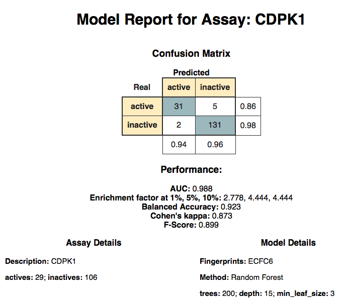
The model report has several elements: the model title, confusion matrix with model performance details, meta information on the data set, and some model details. When we started the parameter optimization we did not know which combination of features, machine learning method, and its hyperparameters would work best for the data set. As it turns out, the best model for our data set was built using Random Forest with 200 trees and ECFC6 chemical fingerprints (param_FPs = 0). The data table from which this Model Report was generated is depicted below and contains the performance statistics of the model along with meta information about the data set and the model parameters.

Figure 6. Fragment of data table used to generate the model report.

We started with a data set and created an automated protocol to select a combination of features and machine learning methods to build the best model for a classification problem, based on a selected criterion. The whole workflow took around 5 minutes to run on a standard machine with 8Gb of RAM allocated to KNIME Analytics Platform. Just enough time to put on a kettle and make yourself a cup of tea. So if you still can't decide which model would be the best for your data set, sit back, relax, and let KNIME pick for you.