A Codeless Approach for Parameter Optimization

What would happen if you put a bunch of data scientists in a room? They’d probably discuss the horrors of parameter optimization. “Why is it so time-consuming? Is it really so important when training a model? Isn’t there a simpler way to find the best parameters?”

To help you tune parameter optimization, we've developed a verified component Parameter Optimization (Table). It computes the best parameters, based on detailed user settings, and visualizes the results. Any machine learning classifier can also be plugged in without much modification.

This article explains parameter optimization, discusses optimization strategies, and walks you through parameter optimization in KNIME, using the verified component. It also points you to a KNIME Hub space: the Parameter Optimization Space. This space includes parameter optimization workflows for you to download and try out.

This is a popular technique to improve machine learning performance. If you are new to parameter optimization, let's briefly review the difference between it and the training of the model itself. Most parameters are learned during the learning phase of model training, but some are set before training begins. These are called hyperparameters. For example, when training a neural network, only the parameter weights in each neuron are improved, in a process called backward propagation. The shape of the network (the number of hidden layers and number of neurons per layer) is fixed before training even begins. In this scenario, parameter optimization means finding the best combination of hidden layers and neurons per layer.

Most data scientists will train a model with the default parameters offered by the adopted machine learning library. When the performance under those defaults is unsatisfactory and no more data can be added to the training set, it is often necessary to optimize those parameters to maximize the model's performance. They can manually choose the parameters, or try different combinations within a range based on their expertise. It becomes challenging as the number of parameters grows in size and each has different ranges. This makes finding the best combination a complicated and time-consuming task. A deeper understanding of the machine learning algorithm is necessary for this.

For example, with the random forest method of classification, parameters like the number of trees and the tree depth need to be optimized. The number of trees may range from 10 to 200, while the depth ranges from 2 to 10, and so on. The right number and depth of trees will yield optimal results.

Even when it is clear which parameters and ranges should be optimized, adopting a naive approach via automatically testing all possible combinations can be computationally expensive. When performing automated parameter optimization, you train the model several times with different combinations. After one iteration, the next combination is picked by a heuristic we call “optimization strategy.” There are a few widely used strategies:

• Random Search - The objective function is evaluated by selecting a random combination of parameters. This method can be beneficial when some parameters have a greater impact on the objective function than others.

• Bayesian Optimization - A random set of parameters is chosen, and the region around the parameters with higher values for the objective function is explored further using the posterior distribution.

• Brute Force - To identify the best parameter combination, all possible combinations within the given range are analyzed.

• Hillclimbing - A random set of parameters is chosen, and in the next iteration, the best from its nearby parameter space are chosen. If none of the parameters improve the objective function, the optimization loop is terminated.

To read more about these strategies, and understand pros and cons, check out “Machine learning algorithms and the art of hyperparameter selection” on the KNIME Blog.

Consider a scenario in which you need to build a classification model for your organization and optimize its performance, but you’re facing a tight time constraint. You are asked to build a classification model on a dataset of satellite images to be classified by soil type (red, gray, damp, and so on). For this example, we use the Statlog (Landsat Satellite) Data Set from UCI ML Repository, where each image is presented in 36 columns describing the different pixels.

First we build a simple solution in KNIME wherein a model is trained with default parameter values without the use of an optimizer. In the KNIME workflow (Figure 1), we’ll use a neural network model (Rprop MLP Learner and Predictor node) for this classification task.

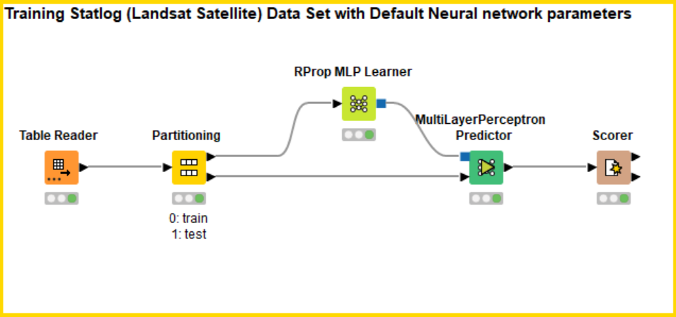
To check the performance of the model, accuracy was selected as the objective metric in the Scorer node. The input of the Scorer node will be the predictions on the test set partition. The output shows a decent accuracy, but can be improved with different parameter combinations. Let's now examine various scenarios for parameter optimization in KNIME.

KNIME offers plenty of nodes for parameter optimization to be performed efficiently and without overfitting. First we are going to see how to optimize the parameters of this neural network model using KNIME Optimization Extension loop nodes.

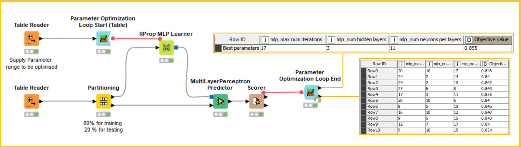
The Parameter Optimization Loop Start (Table) node in KNIME can be used, along with a few additional nodes, to automate the selection of the optimal parameters. This is illustrated in Figure 2, where the neural network is used as the classification model. To adopt this loop node, we provide the list of parameters and possible range of values as an input table. The optimization approach needs to be provided in the setting of the node. In our case, we adopted Bayesian optimization.

We connect the output of the loop node to the learner-predictor workflow segment (Fig. 2). We then open the Flow Variable Panel of the Learner node to select which parameter should be overwritten from the flow variable. To learn more about flow variables, read “KNIME Flow Control Guide.” We then add a Scorer node to evaluate performance in a single iteration, and connect the Parameter Optimization Loop End node and configure the performance metric column to be maximized or minimized.

The first output provides the best parameters to retrain our model. All the parameter combinations and the metric value used for the optimization can be obtained in the second output.

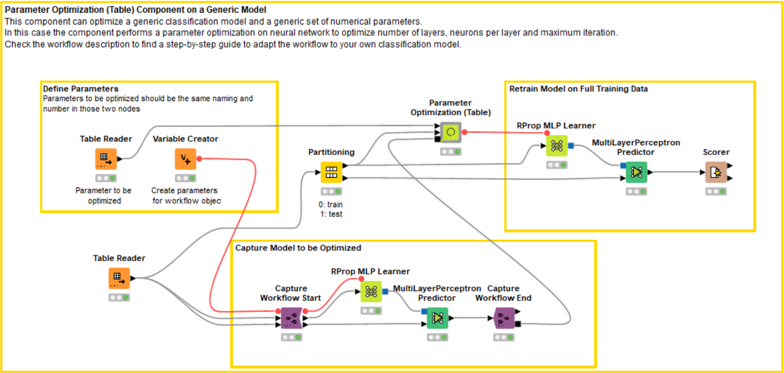
Our verified component can be used to further simplify this process, allowing you to test different classification models to determine which one best fits your data. The component helps you perform this task with cutting-edge techniques (such as Bayesian optimization and nested cross validation) in just a few clicks, saving days of work with a few standardized steps.

Even without extensive understanding of different KNIME nodes, the optimization process is way more simplified by the new Parameter Optimization (Table) component. Some advantages of utilizing the new component:

• Optimize your model with minimum effort. You can simply provide a table that specifies the range each parameter should fall within during the optimization process.

• Training multiple models without much changes to the workflow. By defining the learner and predictor nodes in the workflow segment captured with KNIME Integrated Deployment Extension, the user can apply various classification models to their data.

• Performing Cross Validation. The component adopts the X-Partitioner node to perform a cross validation in each iteration of the parameter optimization loop. This ensures that the performance of a single parameter combination does not overfit the sample.

• Interactive analysis of different parameter combinations. The interactive view displays the best parameters, showing how the performance metric varies over different iterations.

After selecting the ideal parameters using cross validation and the user-provided optimization method, the component generates an output flow variable with the optimized parameter values. This can be used to retrain the model to enhance performance.

To let the component optimize the same neural network of the previous example (Fig. 2), we need to first capture the learner-predictor segment. In Figure 3, you can see the same MLP nodes captured between those purple nodes. Please also notice that a variable from the Variable Creator node is passed to configure the learner node flow variable panel.

The model information is sent to the component using a captured Workflow Port Object. Read more on this type of object in the KNIME blog post “Introduction to Integrated Deployment.”

If you want to change the model — for example, from a neural network to random forest — all you need to do is change the learner and predictor node inside the capture nodes, and make some adjustments to the Table Reader and Variable Creator nodes. This way, you can easily implement parameter optimization on any other model with little modification.

Finally, we are going to show how optimization can be performed on the KNIME Server using the interactive view of the component in a data app.

Up until now, any user optimizing this model would have to download the free and open source KNIME Analytics Platform and adopt our component. Wouldn’t it be better to let any user control the component for a web browser, via a data app. To achieve this, we need to add sliders to control the settings of the parameter search.

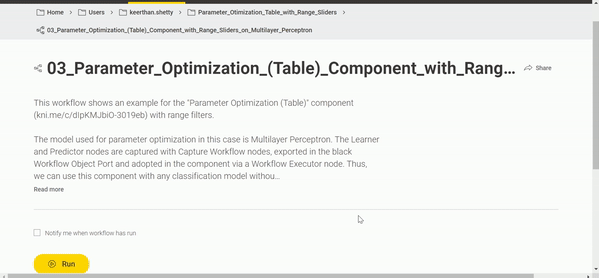
In Figure 4, you can see we added a “Parameter Ranges” component, which lets users decide the range of parameters for the neural network via an interactive view. Inside the component, the Interactive Range Slider Filter Widget node is adopted. The sliders let users select the start and end points for parameter range, as well as the step size for the next parameter (Fig. 5).

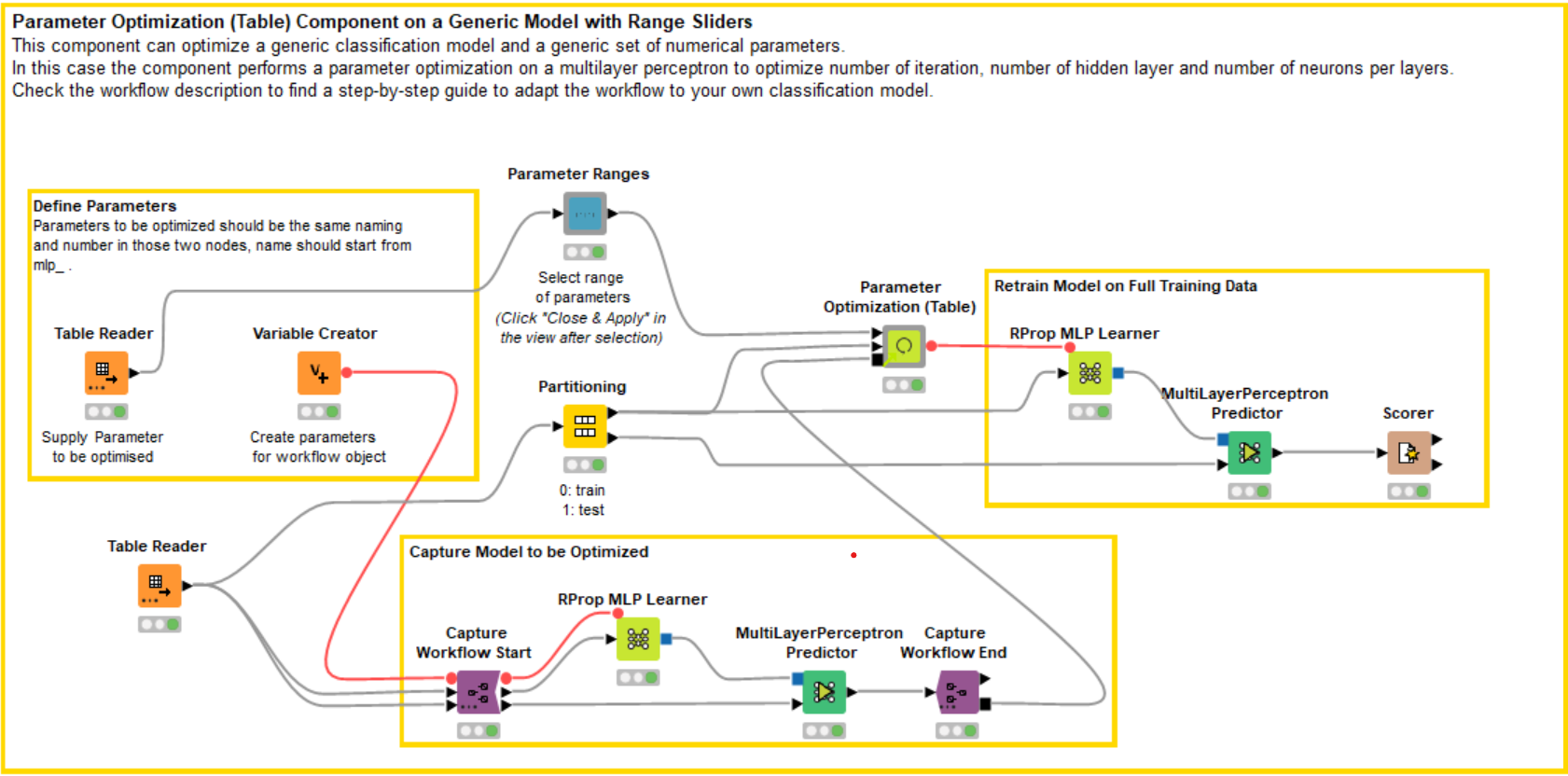
Based on your model and the parameters to be optimized, you can add the right amount of widget nodes to the “Parameter Ranges” component. Once that is done, the workflow can be moved to the KNIME Server, and the data app is then automatically deployed via a unique web browser link. Take a look at the KNIME Data Apps Beginners Guide documentation page to learn more.

Figure 5 demonstrates the workflow of the deployed data app. The user can choose the range and step size for various parameters and experiment with various approaches. Once the parameter optimization is over, a Line Chart showing the results is displayed. On the X axis we see the iterations, and on the Y axis the performance. For our example in Figure 5, we adopted a Bayesian optimization technique, and the graph clearly shows an increasing trend in one performance iteration after another. The winning parameter combination is displayed in the Table View on the right. In our case, that combination clearly comes from the last iterations, where the accuracy oscillates around 0.8568. The graph can be further examined through interactive selection. Each data point represents one combination of parameters — when inspected, they appear in a Tile View below.

In this post, we discussed techniques for parameter optimization. First we developed a neural network classification model using default parameters. Then we optimized a neural network using KNIME Optimization Extension loop nodes. Then, to simplify the process, we showcased how to perform parameter optimization using the new Verified Component Parameter Optimization (Table) with a few standardized steps. Finally, we showed how to deploy the workflow as a data app on the KNIME Serve. The whole parameter optimization can then be controlled from a web browser by any user with access to a unique link.

We published the Parameter Optimization Space for you to experiment and learn via a set of example workflows that can be adapted to your own classification model. In the space, you can find examples for both KNIME Optimization Extension loop nodes and the Verified Component.