PMML, Ensembles and KNIME are three hot topics, each one worthwhile to be used. However, when combined together these three pieces offer an even more powerful approach to data analytics than each one alone. We would like to take the opportunity in this post to tell you more about these three puzzle pieces and, more importantly, about how to put them together.
The puzzle pieces
PMML is THE standard format to represent data mining models. It was first released in July 1997 with version 4.2 having just been published relatively recently in February 2014. The Data Mining Group association is a consortium of companies, including Zementis, SAS, IBM, and of course KNIME, which oversees the definition of the standard format. PMML format is written in XML, which makes it easy to read and understand. One of the strongest advantages of PMML is the portability of predictive models across different analytics tools. With PMML you can generate your model in R, edit it in KNIME, and run it for predictions in the ADAPA cloud.
Ensembles borrow the idea of the “wisdom of the crowd”. If you ask just one expert, the chance of he or she alone failing is generally higher than asking everyone in your network and taking the most frequent – or average – answer. In the case of ensembles, the expert is an advanced learner and the friends in your network are the base learners. Ensembles combine multiple base learners into one powerful ensemble predictor.
KNIME is the last part of this puzzle, and since you are reading this blog, you are probably already familiar with it. If this is not the case, have a look at the KNIME Learning Hub, where you can find tutorials and other learning material to start with KNIME. Now let’s take the puzzle pieces and combine them together! First, we train a single decision tree and export it as a PMML model. Then we train an ensemble of decision trees and also export it as a PMML model. For both examples, we used the Breast Cancer Data Set, which is available online at the UCI Machine Learning repository. The smaller data set we used consists of 8 numerical attributes describing benign and malignant tumors. The goal is to predict the type of tumor on the basis of the input features of the data set.
Creating and evaluating simple and ensemble PMML models in KNIME
Using a Decision Tree Learner node, we build a simple decision tree model to perform the required classification. First, a File Reader node reads the data into KNIME, then a Partitioning node splits the data into training and test set, and finally, a decision tree is trained on the training set only. This is where PMML comes into the picture. The blue squared output port of the decision tree contain PMML documents. You can further edit or extend the PMML documents using XML extension nodes, for example.

To predict the tumor type using the previously learned decision tree, we use the general PMML Predictor node. After the classes have been predicted for each data row in the test set, the Scorer node measures the model performance. The decision tree produced results to a 95% accuracy level, which is a more than acceptable value.
Notice that the PMML Predictor node applies to all PMML models supported by KNIME, be they decision trees or Naïve Bayes or neural networks. Also notice that the same functionality provided by the PMML Predictor node can be found in the JPMML extension nodes in the KNIME Labs section.
Usually, model accuracy can be improved by shifting from a simple decision tree to an ensemble of decision trees. All we need to do is slightly modify the workflow in Fig. decTreeWorkflow.png to train an ensemble of decision trees rather than a single decision tree.
In this example, we build the ensemble through “bagging”. Bagging is a learning technique that trains a number of base models on disjoint subsets of the training set. At the end the base models are combined into one ensemble model. The Chunk Loop Start node generates 20 training subsets and trains 20 decision tree on each one of them; the PMML Ensemble Loop End node collects and combines these 20 base models into one single ensemble model; the PMML Ensemble Predictor node applies all 20 models to each data row in the test set and selects the final class based on a majority vote; finally the Scorer node measures the ensemble performance. The Scorer node indicates a small increase in accuracy from 95% to 96.35%.
Notice that the simple PMML Predictor node cannot deal with ensemble models. Here you need to use the PMML Ensemble Predictor node to implement the majority vote.

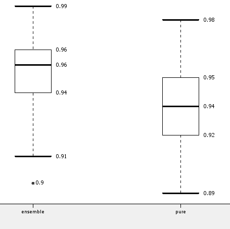
However, as for most data mining algorithms, selection of the training subsets is crucial for the final result. In order to generate a more robust evaluation of the ensemble vs. the single decision tree, we ran both workflows multiple times on shuffled versions of the original data set. The box plot in the following figure shows the mean and standard deviation of the accuracy for the ensemble and for the single decision tree model, confirming the small gain in accuracy when using the ensemble model.

These two small example workflows show that all models produced by KNIME learner nodes, including ensemble models, follow PMML standards and that a special PMML Predictor node is available to apply the majority rule when running ensemble models.
More details about implementing PMML Ensembles models and the PMML Ensemble Predictor node are available in a paper published at the KDD 2013 PMML Workshop.
For more details about the nodes available in KNIME to create and modify any PMML model, the recorded video of a webinar aired on May 6 2014 about PMML and KNIME is now available on Youtube. The KNIME workflow used to create the models and plot can be found in the attachement section of this post.
