Pepper Your Metabolomics Analysis with KNIME

Identifying and quantifying metabolites and small molecules is a key challenge in drug discovery and metabolomics. The search for new drugs in ever-increasing synthetic or natural products databases from different organisms requires a high-throughput method to efficiently screen the compound space.

The food and perfume industries also benefit from the quick discovery of interesting metabolites in a large sample. In recent years, mass spectrometry has evolved to become one of the most important techniques to address this problem. Other research areas, like proteomics, also rely on mass spectrometry, and we discussed its challenges in another article on how to maximize research gains with proteomics analysis.

In this blog post, we will analyze and evaluate a set of publicly available mass spectrometry data for samples of black pepper extract to identify and quantify small molecules.

Black pepper, especially its key alkaloid piperine, facilitates digestion, has protective gastric functions, and plays a role in liver protection and the bio-absorption of micronutrients, vitamins, and trace elements. It helps increase the bioavailability of many types of drugs and phytochemicals.

To screen for other bioactive compounds, so-called untargeted metabolomics experiments through liquid chromatography-coupled mass spectrometry can be performed. One such experiment is available here. It also contains expected locations and relative concentrations of a few hundred compounds that were validated manually or via so-called targeted approaches (under the “Metabolites” tab).

We will use these validated samples to build and demonstrate a successful untargeted metabolomics pipeline in KNIME.

The steps for relative quantification of unlabeled molecules across multiple samples are very similar, independent of the type of molecule:

1. Finding interesting features in retention time and mass-to-charge dimension

2. (Retention time) Aligning mass spectrometry runs

3. Linking corresponding features

4. Quantification

5. Identification

6. Aggregating quantities for the same identity

When working with metabolites or small molecules in general, there are a few important details to consider compared to macromolecules like peptides and proteins. Those differences arise due to the much higher variability of potential structures for the same mass in a candidate pool. While proteins and peptides are linear sequences of amino acids, small molecules can have any structure connecting the chemical elements they consist of, as long as they satisfy a set of rules (e.g., valency rules or sterical/electrical rules). In the paragraphs below, we will highlight specifics for metabolomics applications while going through the key points of the metabolomics pipeline.

Here is an overview of the complete pipeline:

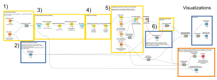
1. The data comes from a server at the University of Tübingen in the open mzML format. We download it automatically using the HTTP Connector, specifying the files to be downloaded in the Table Creator. By default, a subset of the full data is loaded to decrease complexity.

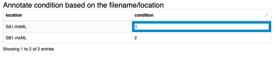
2. We annotate the input data to comply with the experimental design. We specify which files correspond to which condition via the interactive Table Editor node wrapped in the Annotate conditions for files component (Fig. 1).

3. We start the actual data processing with feature finding via the FeatureFinderMetabo node. Its algorithm tries to find interesting regions that look like isotopic mass traces of the same compound in the mass over charge (m/z) and retention time (RT) dimensions. This is done without the knowledge of potential compounds and their locations (Fig. 2). Quantification also happens in this node, by summing all signals that belong to a found feature. We will use the mass-to-charge ratio and retention time of the highest peak in its monoisotopic trace as the location/position of a feature.

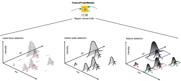
Hint: In the configuration dialogue of this node, important settings like the minimum intensity of a feature or a minimum signal-to-noise ratio can be manually adjusted.

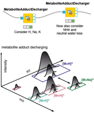
When dealing with metabolites, one should also consider that different features may arise from the same molecule, with different charges and/or adducts. Adduct groups can be found as similar features with certain mass distances, and can help in future steps like alignment and identification. We assign adducts to the features in two sequential MetaboliteAdductDecharger nodes by considering the most likely adducts first (Fig. 3).

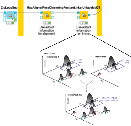
4. Now we need to make sure that we only compare the intensities of features of the same molecule with the same adduct and charge state across files. To correct for potential differences in the chromatography between separate mass spectrometry runs, we align retention times by looking for the most common shifts in the MapAlignerPoseClustering node. After that, in addition to a retention time tolerance, we are using charge and adduct information for quality threshold clustering-based linking in the FeatureLinkerUnlabeledQT node (Fig. 4).

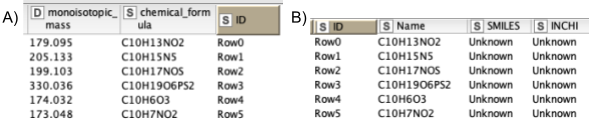
5. Next, we are interested in feature identification, like which molecules the linked features correspond to. We should limit the chemical space to be searched to a smaller number of plausible compounds. Usually one would use specific databases for the types of compounds one is interested in, like the Human Metabolite Database, databases for natural products, or MassBank or Pubchem. For our dataset, we have created a custom database of the compounds available that were identified through other means. Unfortunately, only molecular formulas were provided for each compound. For the AccurateMassSearch node, we need to generate two CSV files (Fig. 5):

• One that maps from the accurate mass of a molecule to IDs of compounds with that mass (Fig. 5A).

• One that maps from ID to properties of the compound like SMILES, trivial name, and more (Fig. 5B).

Based on the average mass-to-charge of features across runs and their potentially annotated adduct, the AccurateMassSearch node then assigns molecules from the database according to a very small mass tolerance.

Note. Keep in mind that even with a very small tolerance, you can have quite a few potential matches per feature. The AccurateMassSearch node will by default perform filtering based on the observed isotope patterns, since specific elements may lead to very distinctive ones due to their particular distribution of natural occurrence.

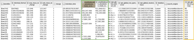
The output of the AccurateMassSearch node is a mzTab file (a table-based file with multiple tables), which we then load with the mzTabReader node into a KNIME table. Only the metadata and the small molecule section will be filled in metabolomics experiments. The small molecule section contains one row per putative identification. Multiple identifications may arise from the same feature if they all fell into the tolerance window. This is evident in the table when multiple identifications have the same mass to charge ratio and retention time, or simply the same opt_global_id_group (Fig. 6, yellow box) value. Intensities in the different input files are stored in the smallmolecule_abundance_study_variable[n] columns, whose order follows the order of the input files (Fig. 6, green box).

6. With the output from the AccurateMassSearch node, we compute changes in intensities of molecules across samples. The simplest way of distinguishing compounds that change notably between conditions is a fold change cutoff, i.e. a threshold on the ratio of the average intensity across conditions. To specify which two conditions to compare to compute those fold changes, we introduced a component Choose comparison for interactive selection from all specified conditions. The aggregation and ratio calculation then happens in a set of KNIME nodes in the Compute fold changes metanode.

Note. In natural products research, this allows us to compare, for example, the yield of different extraction methods or different plants. In crop sciences, this can be used to determine the origin of expensive crops like asparagus or truffles by comparing whole intensity profiles of multiple compounds taken up through the soil.

For every mass spectrometry analysis, one would like to check whether the identification was done correctly and if any peaks were missed, and explore the extracted intensities of the detected signals. For our example dataset, we are in an advantageous position to evaluate the performance of the workflow, because the dataset contains a set of spiked-in and manually validated compounds.

Since multiple assignments of compounds to features within a certain threshold are possible, we are going to pick the closest match for each feature via a set of nodes in the Find closest match to expected compounds metanode. Then we calculate the deviations of the feature’s position to the expected location, as well as the error in the expected fold change. We display the results in a set of violin plots divided into common adducts to see if there is a bias in the accuracy dependent on the type of adduct (Fig. 7).

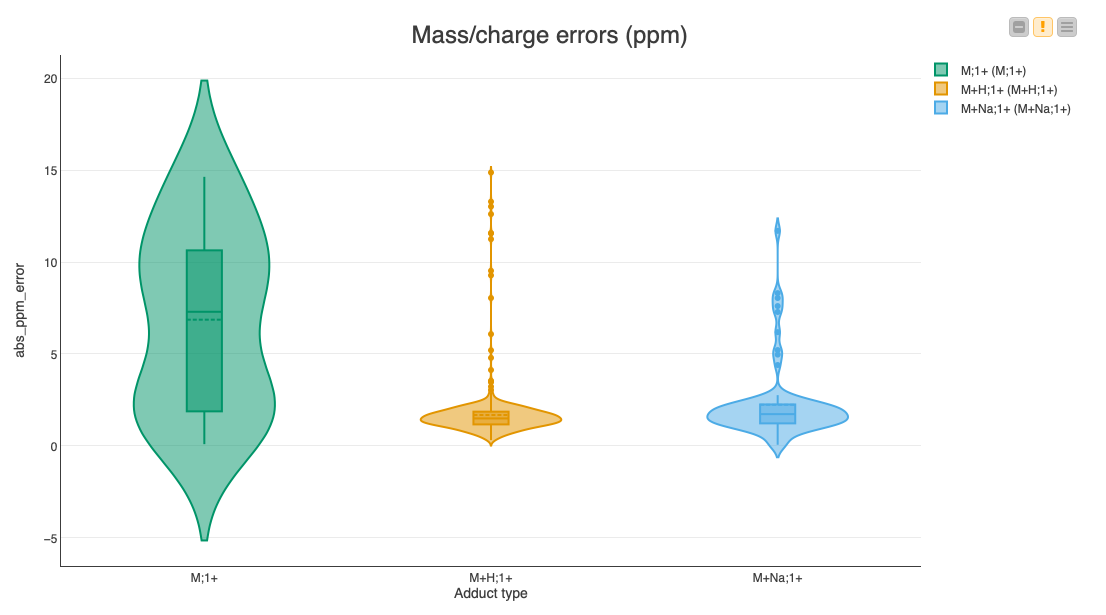
The median errors of the common adducts like a proton or a sodium ion are very low (less than 2 ppm). However, the errors of the inherently charged molecules without adducts sometimes reach our maximum allowed threshold of 20 ppm, indicating that it might be a false assignment to the found feature.

Next we investigate whether any expected features were either not found or not identified via the Calculate missing metabolites metanode and the Create table of pictures at places with missing compounds component, respectively. We extract data with the pyopenms package, which allows efficient reading and processing of raw mass spectra and the intermediate results from the OpenMS nodes. In our dataset, we see three reasons for missing features (Fig. 8).

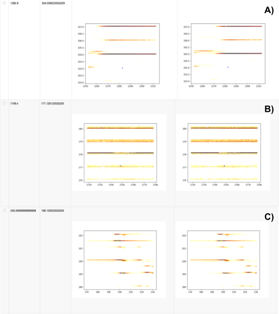
We show three different cases:

1. No signal found, either due to wrong ground-truth annotations (unlikely) or very low intensity signals that became invisible due to the interpolation used for plotting.

2. Features in very noisy regions that will be hard to identify, independent of the parameters used for feature finding.

3. Features of decent shapes that can probably be found with additional parameter tuning (e.g. lower the considered signal-to-noise ratio in FeatureFinderMetabo).

The regions can alternatively be exported with the CSV Writer to be inspected interactively in an external viewer such as TOPPView.

Lastly, we provide an interactive visualization that allows us to explore differences in quantities of the identified molecules across conditions in the Table View with PubChem Browser component. It can be used with any dataset.

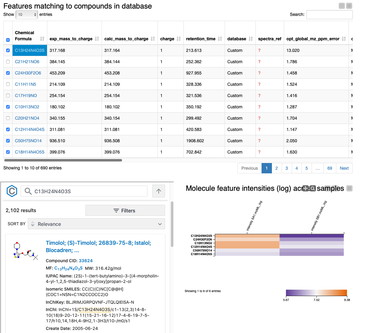
The summary table and the heatmap contain one row per feature, with their closest molecular formula annotated and arbitrarily resolved if there were ties. We can identify the compounds that change the most across conditions by sorting the table according to fold change. We also added a small PubChem lookup inlet to get a glimpse of possible structures and additional information by clicking on the chemical formula of a row. The table should include everything you need for the successful discovery of the interesting compounds you are looking for. Extensions to the pipeline after this point might include normalization, imputation, statistical significance testing, and/or clustering compounds by their fold change profile.

Note that fractionated samples (i.e., samples that underwent additional separation before the mass spectrometer) are not yet supported by the workflow. Under such circumstances, the workflow would need to be executed once for every fraction. You might have noticed another important problem already: “Aren’t there many compounds with the same molecular formula? How do I know which is the right one in the PubChem lookup?” Unfortunately, finding the correct structure for an unknown feature is much more difficult, and requires the integration of information from isotope patterns, adducts, and additional information like fragment spectra, which are not present in this dataset. We will therefore tackle this problem in a follow-up post, which will build on many of the concepts shown here.