
A CHEMBL-OG post, Multi-task neural network on ChEMBL with PyTorch 1.0 and RDKit, by Eloy, from way back in 2019 showed how to use data from ChEMBL to train a multi-task neural network for bioactivity prediction - specifically to predict targets where a given molecule might be bioactive. Eloy has links to more info in his blog post, but multi-task neural nets are quite interesting because the way information is transferred between the different tasks during training can result in predictions for the individual tasks that are more accurate than what you’d get if you just built a model for that task alone.
It’s a big contrast to most humans: our performance tends to go down the moment we start multitasking. In any case, I find this an interesting problem and Eloy provided all the code necessary to grab the data from ChEMBL and reproduce his work, so I decided to pick this up and build a KNIME workflow to use the multitask model. For once I didn’t have to spend a bunch of time with data prep (thanks Eloy!) so I could directly use Eloy’s Jupyter notebooks to train and validate a model. After letting my workstation churn away for a while I had a trained model ready to go; now I just needed to build a prediction workflow.
Loading the Network and Generating Predictions
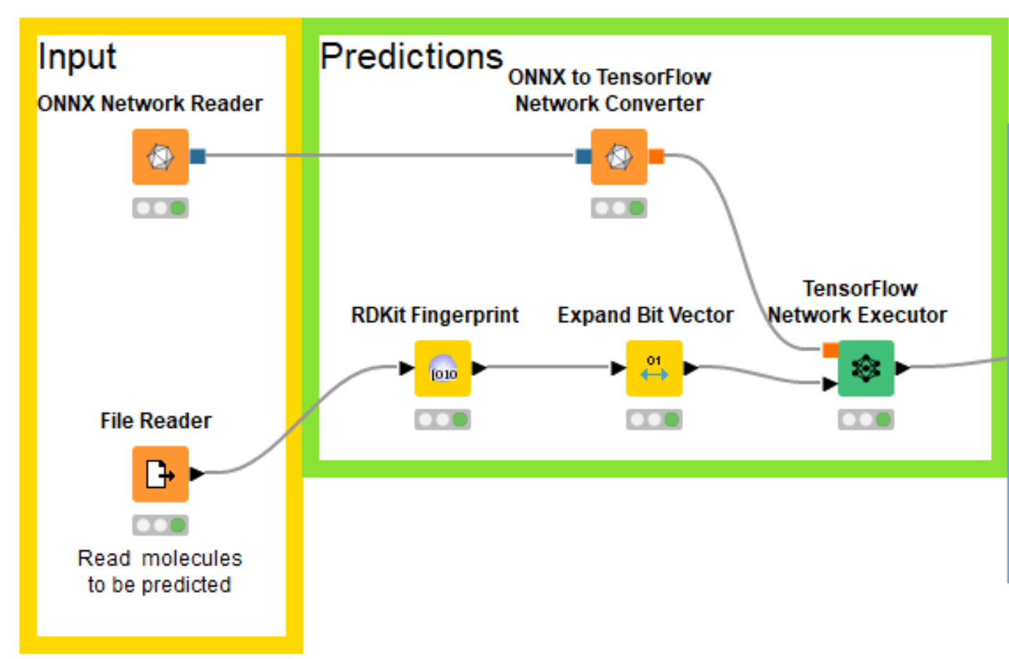
Eloy’s notebooks build the multitask neural network using PyTorch, which KNIME doesn’t directly support, but fortunately both KNIME and PyTorch support the ONNX (Open Neural Network Exchange https://onnx.ai/) format for interchanging trained networks between neural network toolkits. So I was able to export my trained PyTorch model for bioactivity prediction into ONNX, read that into KNIME with the ONNX Network Reader node, convert it to a TensorFlow network with the ONNX to TensorFlow Network Converter node, and generate predictions using the TensorFlow Network Executor node.
Now that I have the trained network loaded into KNIME, I need to create the correct input for it. Since the model was trained using the RDKit this is quite easy using the RDKit KNIME Integration.
Interested in finding out more about using the RDKit, KNIME and Python for advanced chemistry? Watch a recording of Greg Landrum's webinar "Advanced chemistry: RDKit + KNIME + Python for the win", where he showed how this blend of tools is used together for complex R-group analysis.
Watch a video of the webinar on our KNIME TV YouTube channel here
I know that the model was trained using the RDKit’s Morgan fingerprint with a radius of 2 and a length of 1024 bits and I can generate the same fingerprints with the RDKit Fingerprint node. Since I can’t pass fingerprints directly to the neural network, I also add an Expand Bit Vector node to convert the individual bits in the fingerprints into columns in the input table. The compounds that we’ll generate fingerprints for are read in from a text file containing SMILES and a column with compound IDs that we’ll use as names. The sample dataset used in this blog post (and for the example workflow) is made up of a set of molecules exported from ChEMBL and a couple of invented compounds I created by manually editing ChEMBL molecules.
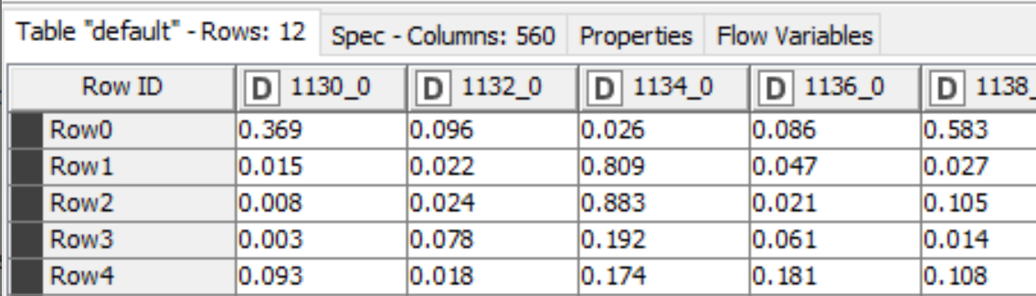
The output of the TensorFlow Network Executor node is a table with one row for each molecule we generated a prediction for and one column for each of the 560 targets the model was trained on. The cells contain the scores for the compounds against the corresponding targets, Figure 2.
At this point we have a pretty minimal prediction workflow: we can use the multitask neural network to generate scores for new compounds. In the rest of this post I’ll show a couple of ways to present the results so that it’s a bit easier for people to interactively work with them.
Showing the Predictions in an Interactive Heatmap
The first interactive view that we’ll use to display the predictions from the multitask neural network includes a heatmap with the predictions themselves and a tile view showing the molecules the predictions were generated for. The heatmap has the compounds in rows and targets in columns with the coloring of the cell determined by the computed scores. The tile view is configured to only show the selected rows.
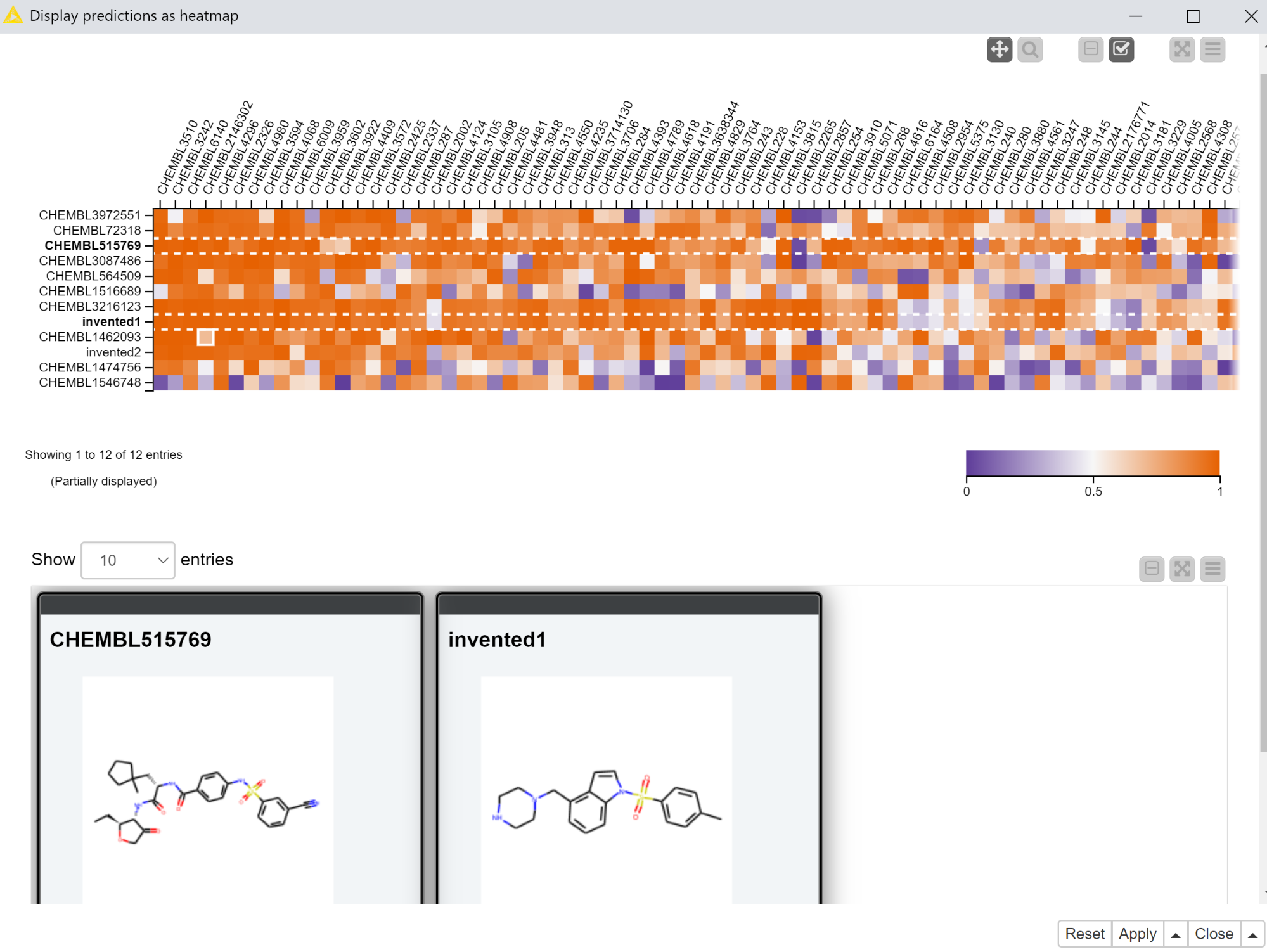
The “Display predictions as heatmap” component that exposes this interactive view is set up so that only selected rows are passed to its output port. So in the example shown in Figure 3, there would only be two rows in the output of the “Display predictions as heatmap” component.
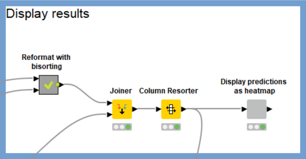
The workflow does a significant amount of data processing in order to construct the heatmap. I won’t go into the details here, but the main work occurs in the “Reformat with bisorting” metanode, which reorders the compounds and targets based on their median scores. This brings targets which have more high-scoring compounds to the left of the heatmap and compounds with high scores against more targets to the top of the heatmap. Qualitatively the heatmap should get more red as you pan up and to the left and more blue as you pan down and to the right. There’s no best answer as to the best sorting criteria for this purpose, so feel free to play around with the settings of the sorting nodes in the “Reformat with bisorting” metanode if you’d like to try something other than the median.
Comparing Predictions to Measured Values
A great way to gain confidence in a model’s predictions is to compare them with measured data. Generally we can’t do this, but sometimes there will be relevant measured data available for the compounds we’re generating predictions for. In these cases it would be great to display that measured data together with the predictions. The remainder of the workflow is there to allow us to do just that, Figure 5.
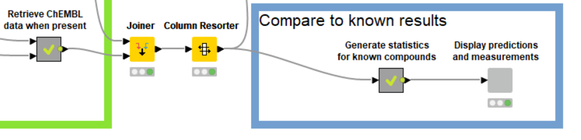
This starts by generating InChI keys for the molecules in the prediction set, looking those up using the ChEMBL REST API, and then using the API again to find relevant activity data that was measured for those compounds. Daria Goldman wrote a blog post, entitled A RESTful way to find and retrieve data a couple of years ago, showing how to do this. I’ve tweaked the components she introduced in that blog post for this use case and combined everything in the “Retrieve ChEMBL data when present” metanode.
The output table of the metanode has one row for each compound, a ChEMBL ID for each compound that was found in ChEMBL, and one column for each target where there was experimental value in ChEMBL for one of the compounds in the prediction set. This data can be visualized, together with the predictions using the “Display predictions and measurements” component, Figure 6.
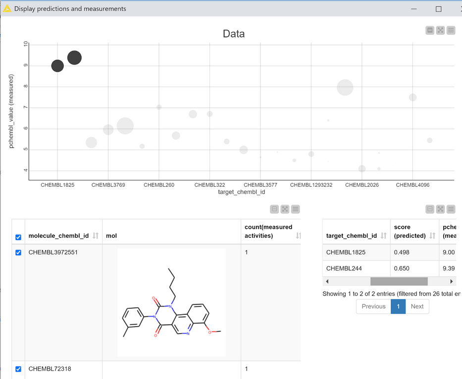
This interactive view is primarily based on the scatter plot at the top. Each point in the plot corresponds to one compound with data measured against one target. The CHEMBLIDs of the targets are on the X axis and the measured pCHEMBL values (as provided by the ChEMBL web services) are on the Y axis. The size of the points in the plot is determined by the calculated score of that compound for that target. The scatter plot is interactive: selecting points shows the relevant compounds in the table at the bottom left of the view and the corresponding scores and measured data in the table at the bottom right.
If the model is performing really well I’d expect the scatter plot in Figure 6 to have large scores (big points) for compounds which have high activity (large pCHEMBL values), i.e. bigger points towards the top of the plot and smaller points towards the bottom. That’s more or less what we observe. There are clearly some outliers, but it’s probably still ok to pay at least some attention to the model’s predictions for the other compounds/targets. (Note: This isn’t a completely valid evaluation since most of the data points I’m using in this example were actually in the training set for the model. The example is shown here in order to demonstrate the view and its interactivity.)
Wrapping Up
In this blog post I’ve demonstrated how to import a multitask neural network for bioactivity prediction built with PyTorch into a KNIME workflow and then use that to generate predictions for new compounds. I also showed a couple of interactive views for working with and gaining confidence in the model’s predictions. The workflow, trained model, and sample data are available on the KNIME hub for you to download, learn from, and use in your own work.