
ABC analysis is a strategic approach to inventory management, optimizing decision-making about which stocks to retain and which to discard. It involves categorizing inventories into three groups, namely A, B, and C, based on their importance to the sales volume. Category A items drive a significant portion of the sales volume, category B items contribute a moderate sales volume, and category C items yield the least sales volume.
The idea of ABC analysis is rooted in Pareto’s Principle, which suggests that 80% of sales come from 20% of items sold. Therefore, categories A and B amount for the most number of sales but from the fewer set of items. Since item category A is critical, it requires special attention and planning by business executives to avoid stockouts.
There are multiple advantages of this analysis, including:
-
Improved inventory control, thus preventing out-of-stock scenarios for crucial items.
-
Cost reduction by concentrating on key items, enhancing profitability.
-
Improved demand forecasting for essential items.
-
Optimized supplier terms to ensure further cost optimization on critical items.
While there are benefits of employing ABC analysis there are also its drawbacks, including:
-
Difficulty in defining clear boundaries between categories, as this often relies on intuition, making accurate item classification challenging.
-
Seasonal variations in demand can lead to inefficient inventory management, despite accounting for demand uncertainty.
Use Case: ABC Analysis of Lamp Sales
The dataset for this use case comprises sales data for different types of lamps sold between January 2022 and June 2022. It includes the price per item and the category of each lamp. Two workflows have been established for ABC analysis:
The first workflow categorizes items by using a basic ABC classification model. This classification categorizes items according to their sales value.
The second one extends from the first one and also implements demand variability in the classification. This is called ABC XYZ analysis or just XYZ analysis.
Workflow 1: Basic (or Naive) ABC Analysis
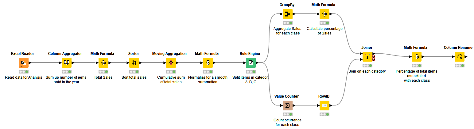
This workflow, which you can download here from KNIME Community Hub, classifies items in one-dimensional criteria - total sales from each category. The steps involved in classifying items are as follows:
1. Calculating total sales for each item for the given period, sorted in descending order.
2. Calculating the cumulative sum of total sales.
3. Converting the cumulative sum of sales into a percentage of the grand total
4. Defining bounds for categories A, B, and C, and categorizing each item into the respective group based on the previously calculated percentage. For this use case, the bounds are set as follows:
-
A ⇒ 0.0 – 0.60
-
B ⇒ >0.6 – 0.85
-
C ⇒ >0.85
Aggregating sales and item count for each category and calculating their respective percentage of the grand total.
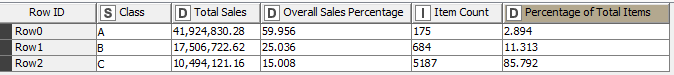
As shown in Fig. 2, 60% of sales come from just 2.9% of items. This shows the importance of category A. Category B follows, which comprises 25% of sales from roughly 11% of items. This shows the medium level of criticality from category B. Finally, category C accounts for 15% of total sales which comes from roughly 86% of items. Therefore, based on sales volume calculated for six months, inventory can be planned accordingly for the next period.
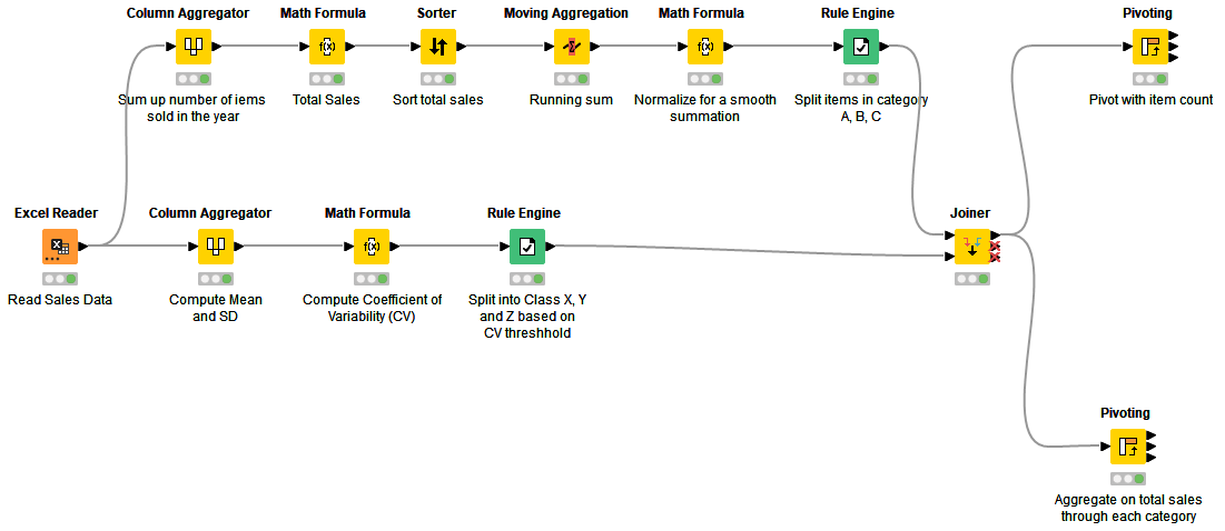
Workflow 2: ABC Analysis with Variability of Demand
This workflow, which you can download here from KNIME Community Hub, extends from the first one and calculates classification with not just respect to total sales but also considers demand variability. The variability measure used here is also called the coefficient of variation (CV) which measures the size of variation from the mean in data.

Consider three sets of numbers:
-
Set 1 : [50, 50, 50, 50] ⇒ S.D () = 0, Mean () = 50 ⇒ CV = 0
-
Set 2: [40, 50, 60, 70] ⇒ S.D () = 11.18, Mean () = 55 ⇒ CV = 0.203
-
Set 3: [1, 10, 135, 835]⇒ S.D () = 344.59, Mean () = 245.25 ⇒ CV = 1.405
From the three sets of numbers, values in set 1 are constant, as a result, it has a standard deviation of 0 and subsequently a CV of 0. In set 2, the variation of figures is in slight proximity with each other, therefore the CV is closer to zero but not equal to zero. However, in set 3 the degree of variation between figures is drastic, therefore it has a CV of greater than 1.
In the workflow, CV is implemented after step 4 from the first workflow:
5. Calculate the mean and standard deviation of each item sold across the period. Calculate the CV from the results in step 5.
6. Assign categories X, Y, and Z to bins based on thresholds from the CV calculated in step 6. For this workflow, bounds for the bins are set as follows: X ⇒ 0.25 – 0.80
7. Merge categories X, Y, and Z with categories A, B, and C to classify item counts and corresponding sales (Fig. 5 & 6).
To better understand it, XYZ analysis accounts for volatility of demand in each categories A, B, and C. Category Z belongs to the most volatile demand and X belongs to the least volatility in demand for each category A, B, and C. CV value of less than 1 is considered to represent stable demand while a value that is greater than 1 tells otherwise. Therefore, inventory management for items along category Z is always challenging for a business to minimize incurring costs.
Below, fig. 4 demonstrates the explanation of each segment in this two-dimensional inventory classification process. For instance, AZ is the most critical in the entire matrix because it contains items that bring in high sales volume and have very fluctuating demand. On the other hand, AX also shows high sales volume but of items that have relatively stable demand.
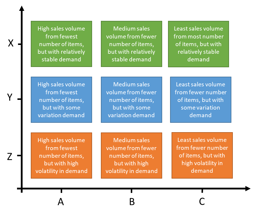
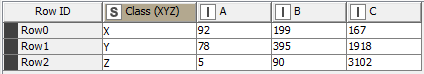
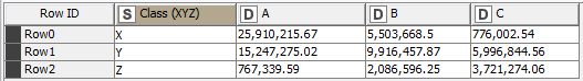
In conclusion, 3102 items from category C generate the least sales volume but are subject to high demand uncertainty (Fig. 5). Only five items from category A, the highest sales category, experience high demand uncertainty (Fig. 5). Category X contributes the highest number of sales from all items in A, B, and C (Fig. 6). This indicates that items yielding the highest revenue have the least variation in demand.
Enabling cost-effective decisions in inventory management
In summary, several approaches can be used for ABC analysis, with some advanced methods also considering demand uncertainty. The primary purpose of this classification is to enable business users to make cost-effective decisions in inventory planning.