We often think of data science as a young field, and in many ways it is. Its widespread application across myriad industries is very much a product of the 21st century. And yet many of the analytical tools we data scientists employ are old.
The poster child for this is the Neural Network, which was first conceived in the 1940s, some 80 years ago. Other techniques we use are older still, such as the Fourier transform. This powerful yet simple operation was originally demonstrated in 1822 — 200 years ago!
What is a Transform?
Transforms are mathematical operations that transform input data into a new representation. A common example is the log transform, which as the name suggests uses the log operation. It can be inverted by applying the exponential operation:
x’ = Log(x)
x = e^x’
Where x is the original data and x’ is the transformed data. (Note that not all transforms are reversible, but it is a useful feature.) Now let’s move on to the transform that we’re really here to see.
What is the Fourier Transform?
Like the log transform, the Fourier transform converts numeric data into a new format. Instead of applying a log operation, it uses this equation:
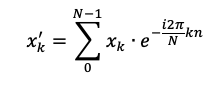
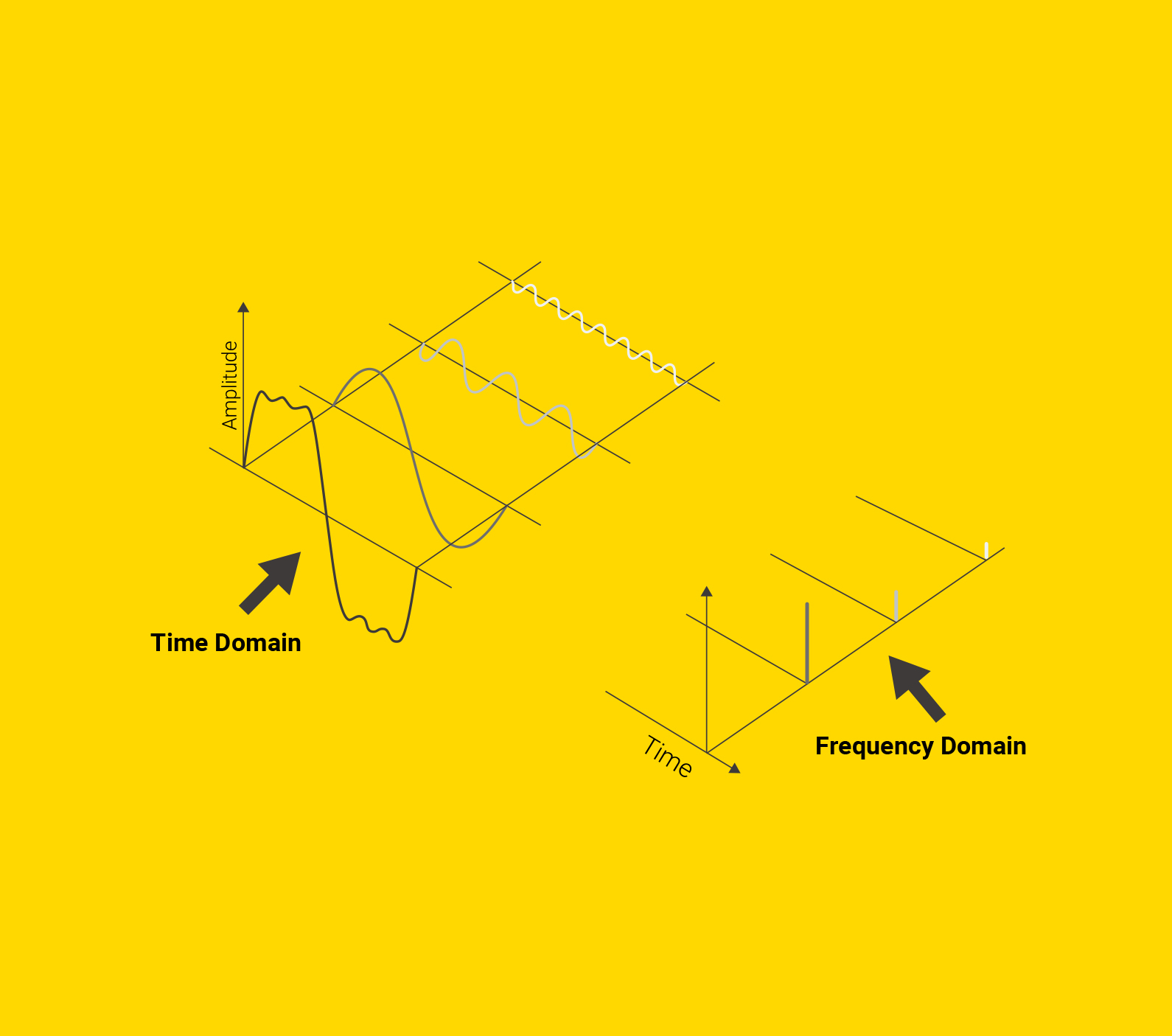
Don’t worry if this equation looks a bit alien to you. While the math behind the Fourier transform can be quite advanced, the concept is simple. If you’ve taken a calculus class, you may be familiar with the Taylor series. This is a method of re-expressing any continuous function as a polynomial. This means we can take a function like f(x) = sin(x) and express it in a more interpretable format. (This is actually how computers are able to perform these types of operations!) Similarly, the Fourier transform re-expresses a function as a sum of sine waves of varying frequencies and amplitudes. Thanks to Euler’s equation, we use the complex exponential — that’s the e with the i in it’s exponent in Figure 1! So how should you picture this transformation?
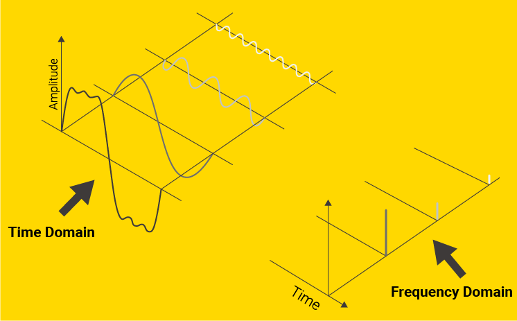
On the far left is some original signal. To the right of it are three sine waves that recreate it when added together. On the far right, we visualize the amplitudes of these component waves, which are the representations of the original data in the frequency domain.
Why is the Fourier transform useful?
Representing time series data in the frequency domain allows us to extract and gauge the strength of different patterns in our data. Take auditory data, for example, like the recording of a musical chord. Applying the Fourier transform to convert that data to the frequency domain allows us to see the frequency and relative loudness of the individual notes.

Furthermore, we could use this technique to detect whether an additional note was played by accident during the execution of the chord.
Where is the Fourier transform useful?
While music is the most familiar auditory data, it is not what makes the Fourier transform so incredibly useful. Vibration and auditory sensors attached to industrial machines, perhaps on a production line, can capture data in a similar format. Sound is just vibration in the air, after all.
Just like how we can note an anomaly in a musical chord when we detect a frequency we did not expect, we can note an anomaly in a machine by detecting a vibration, or indeed sound, we did not expect. To define what vibrations we expect from a machine, we analyze data under normal functioning conditions
How can I use the Fourier transform?
This process can be a lot to wrap your head around, but with KNIME Analytics Platform, you can get through the stages in no time at all!
In this quick example, we have two data sets — one containing data from a normally functioning turbine, and one from a turbine with a bearing that is going bad. We will use only this normal functioning data to “train” our anomaly detector. (“Train in quotes because there is no machine learning model!)
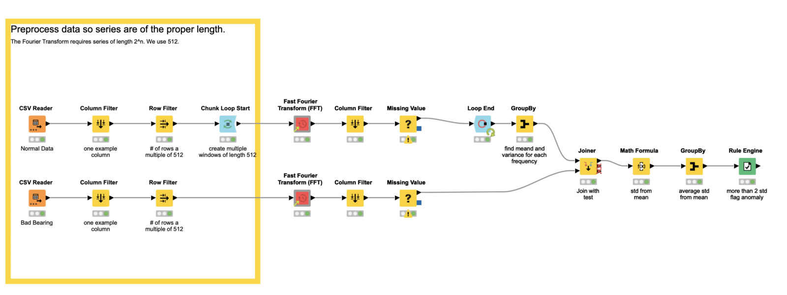
Fig. 4 : Preprocessing data so that our series have the proper length in the example workflow, Fourier Transform for Anomaly Detection, which is publicly for download from the KNIME Hub.
Tip: Download the example workflow, Fourier Transform for Anomaly Detection, from the KNIME Hub
The power of our anomaly detector comes from the Fourier transform. In discrete format, which we will almost always use, we require the length of our series be a power of 2. In this example, we use 2⁹, or 512. To that end, we apply some preprocessing so our total data series is a multiple of 512 — the window size we plan to use in the Fourier transform. (Another option for dealing with the series length requirement is to pad the series with zeroes.)
To create the multiple windows through which we will deploy the Fourier transform, we use the Chunk Loop Start node. It enables us to cut 512 rows at a time out of our data set for processing inside each iteration of the loop body, which we’ll look at next.
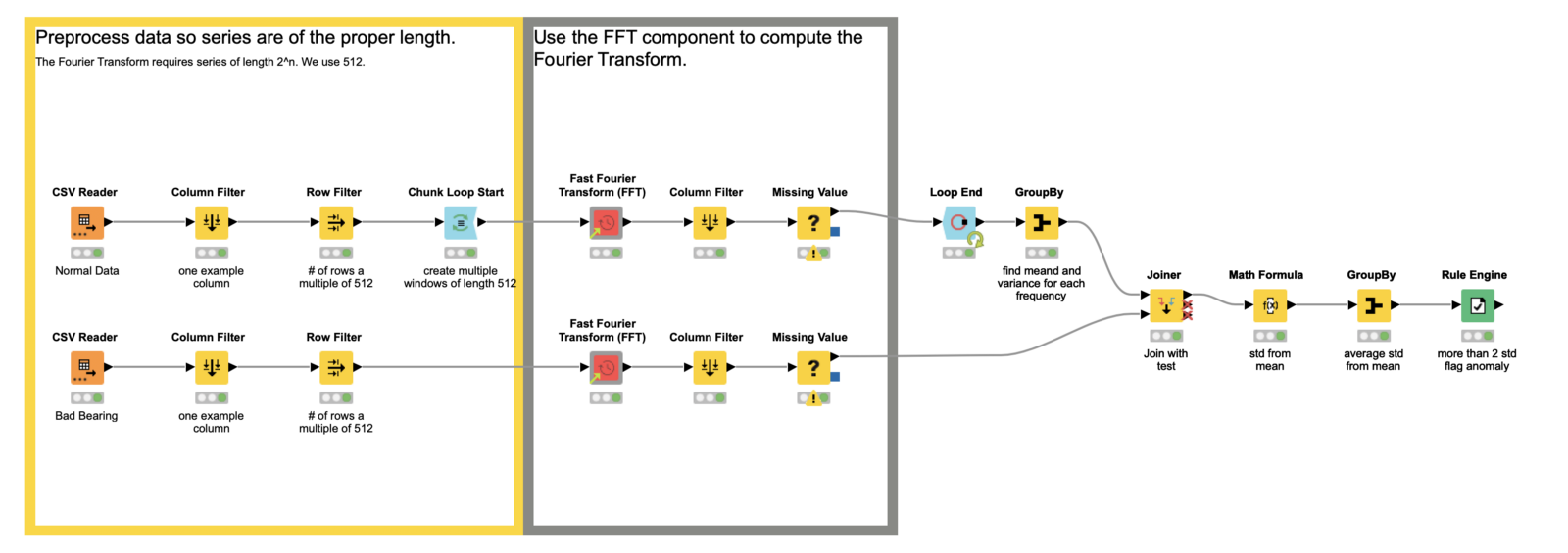
Now that we are inside the loop body, we apply the Fourier transform. However, when we are working with discrete data, which we (almost) always are as data scientists, we use its discrete variation, aptly named the discrete Fourier transform, or DFT. To do this in KNIME, we’ll use the Fast Fourier Transform (FFT) component. It is a set of algorithms that calculate the DFT quickly. You can find it on the KNIME Community Hub, or on the example server under “Components > Time Series”. There’s little else we need to do inside the loop body here; the component takes care of all our Fourier transform needs! There is still some work to be done to build our actual anomaly detector, though.
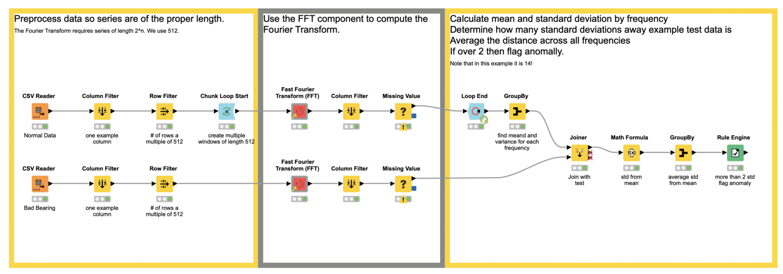
Finally we come to the detection bit! To do this, we aggregate the results of the FFT we applied to the different windows of our normal data. We want both the mean and the standard deviations. We’ll use those in the next step to decide if our test data is anomalous.
So far we’ve applied the FFT on our normal data and extracted the mean and standard deviation for each frequency the transform outputs. Now we join that information to our test data, and in the Math Formula node, we calculate the number of standard deviations each frequency is away from the mean of our test data. We further aggregate those values to see the average number of standard deviations for all our frequencies.
Finally, at the end of the workflow, the Rule Engine node is used to flag anomalies. We simply rule that if our final aggregated term is larger than 2, we have an anomaly. This number can be raised or lowered, based on risk tolerance and other features.
Now Try an Example Workflow using the Fourier Transform Yourself
Here we’ve explored the simple nature of the Fourier transform — it decomposes signals into sine waves of varying frequency. In music, we think of those frequencies as notes. The ability to extract these periodic patterns from a signal is useful when exploring data, making forecasts, or (as seen in our example) anomaly detection. To demonstrate this, we’ve looked at a workflow that, using only the Fourier transform and some aggregation, detects anomalies in Turbofan data. Now try out the example workflow yourself!