How to Detect Outliers | Top Techniques and Methods

Outliers in statistics are unusual or extreme values in a dataset that stand out from the majority of other data points. They typically arise from measurement errors or unique system conditions and don't accurately represent the usual behavior of the underlying system. They can mess up statistical analyses and skew results, so it's important to spot and handle them correctly. 

Moreover, in some cases, outliers can give you information about localized anomalies in the whole system; so detecting outliers becomes a valuable step that enhances your understanding of the dataset. 

How to detect outliers: four detection techniques

There are many techniques to detect and optionally remove outliers from a dataset. In this article, we will explain the four most frequently used - traditional and novel - techniques for detecting outliers:

1. The numeric outlier technique
2. The Z-score method
3. The DBSCAN technique
4. The isolation forest method

We will also show you how to use them in KNIME Analytics Platform with an example.

This is a simple, nonparametric outlier detection method in a one dimensional feature space. Here outliers are calculated by means of the InterQuartile Range (IQR).The first and the third quartile (Q1, Q3) are calculated. An outlier is then a data point x_i that lies outside the interquartile range. That is:

x_i > Q3 + k(IQR)   x_i < Q1 - k(IQR),
where IQR = Q3 - Q1 and k0.

This outlier treatment can easily be implemented in KNIME Analytics Platform using the Numeric Outliers node.

Z-score is a parametric outlier detection method in a one or low dimensional feature space.

This approach assumes a Gaussian distribution of the data. The outliers are the data points that are in the tails of the distribution and therefore far from the mean. How far depends on a set threshold z_thr for the normalized data points z_i calculated with the formula:

z_i=x_i - μ / σ

where x_i is a data point, μ is the mean of all x_i and σ is the standard deviation of all x_i.

An outlier is then a normalized data point which has an absolute value greater than z_thr. That is:

| z_i |>z_thr

Commonly used z_thr values are 2.5, 3.0 and 3.5.

This technique is based on the DBSCAN clustering method. DBSCAN is a nonparametric, density based outlier detection method in a one or multi dimensional feature space.

In the DBSCAN clustering technique, all data points are defined either as Core Points, Border Points or Noise Points.

• Core Points are data points that have at least MinPts neighboring data points within a distance ε.
• Border Points are neighbors of a Core Point within the distance ε but with less than MinPts neighbors within the distance ε.
• All other data points are Noise Points, also identified as outliers.

When discussing how to detect outliers, it is important to note that detection depends on the required number of neighbors MinPts, the distance ε and the selected distance measure, like Euclidean or Manhattan.

This is a nonparametric method for large datasets in a one or multi dimensional feature space.

An important concept in this method is the isolation number.

The isolation number is the number of splits needed to isolate a data point. This number of splits is ascertained by following these steps:

• A point “a” to isolate is selected randomly.
• A random data point “b” is selected that is between the minimum and maximum value and different from “a”.
• If the value of “b” is lower than the value of “a”, the value of “b” becomes the new lower limit.
• If the value of “b” is greater than the value of “a”, the value of “b” becomes the new upper limit.
• This procedure is repeated as long as there are data points other than “a” between the upper and the lower limit.

It requires fewer splits to isolate an outlier than it does to isolate a nonoutlier, i.e. an outlier has a lower isolation number in comparison to a nonoutlier point. A data point is therefore defined as an outlier if its isolation number is lower than the threshold.

The threshold is defined based on the estimated percentage of outliers in the data, which is the starting point of this outlier detection algorithm.

This technique was implemented using the KNIME H2O Machine Learning Integration. 

An explanation with images of this technique is available at https://quantdare.com/isolation-forest-algorithm/.

Let's use the well known airline dataset to test and compare the four outlier detection techniques. The dataset includes information about all US domestic flights between 2007 and 2012, such as departure time, arrival time, origin airport, destination airport, time on air, delay at departure, delay on arrival, flight number, vessel number, carrier, and more. Some of those columns could contain anomalies, i.e. outliers.

From the original dataset we extracted a random sample of 1500 flights departing from Chicago O’Hare airport (ORD) in 2007 and 2008.

In order to show how the selected outlier detection techniques work, let’s focus on finding outliers in terms of average arrival delays at airports. Average arrival delay is calculated on all flights landing at a given airport. We are looking for those airports that show unusual average arrival delay times.

Figure 1 below shows the outlier airports detected by the isolation forest method. The blue circles represent airports with no outlier behavior while the red circles represent outlier airports. The average arrival delay time defines the size of the circles.

Notice that outlier airports are detected in both directions of the arrival delay scale: airports with frequent long arrival delays as well as airports with frequent small or even negative arrival delays. An example of such an airport with a negative average arrival delay (-17 min) is New Orleans Louis Armstrong International Airport.

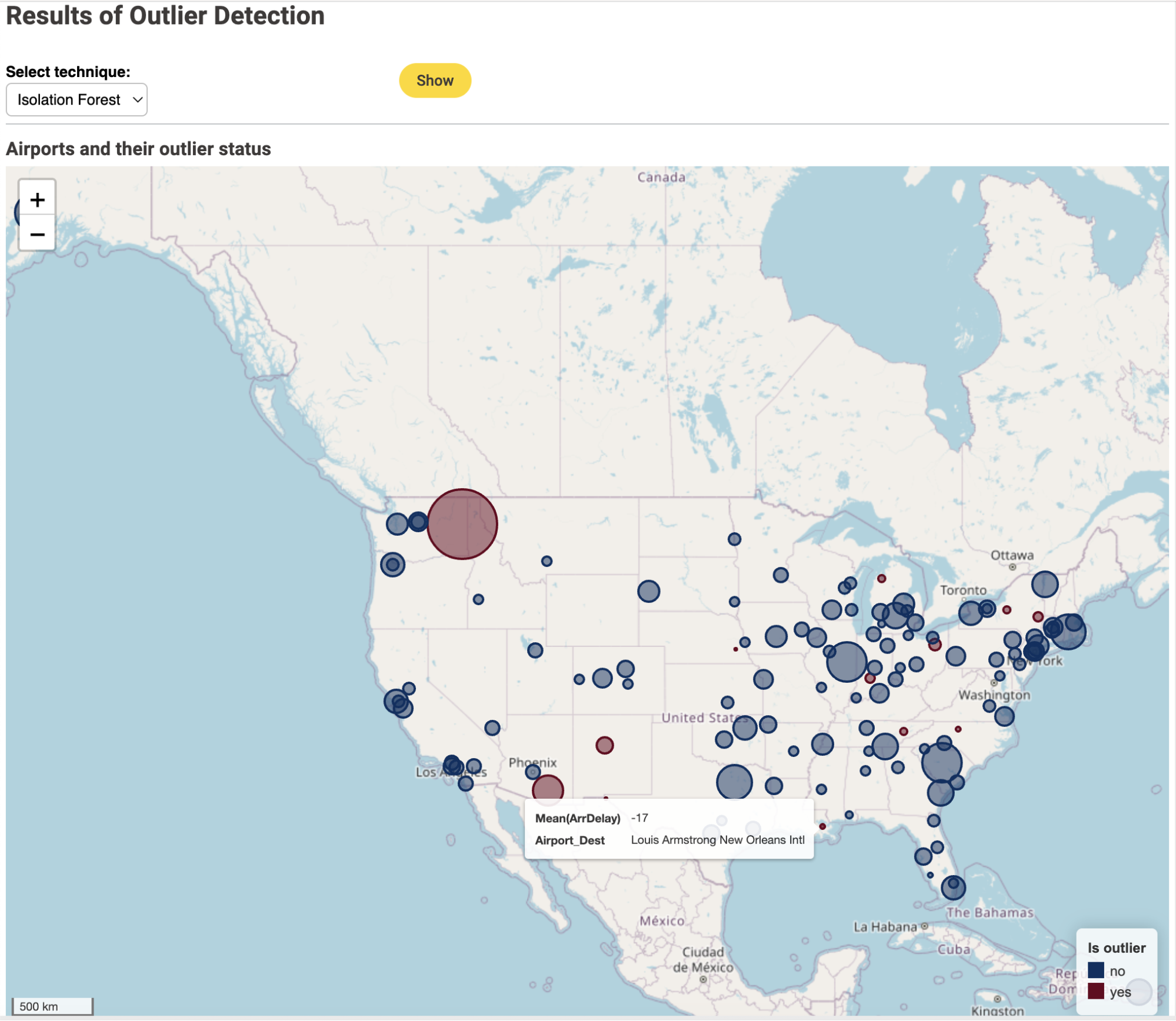
The outlier status of the airports could then lead to a closer inspection of their recording processes and infrastructure.

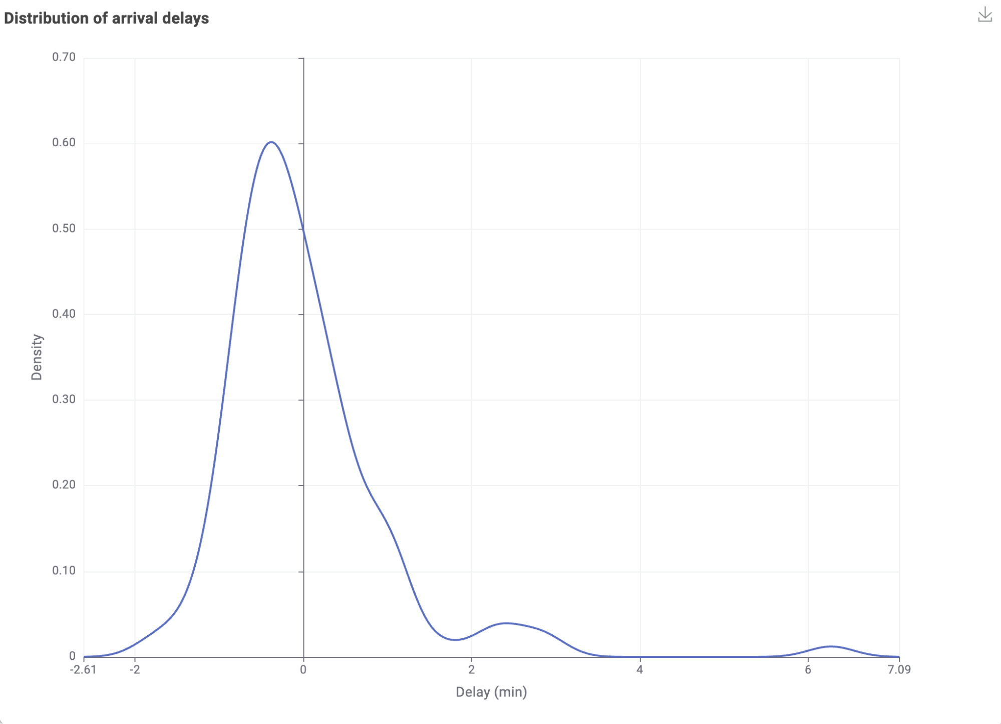
The graph in Figure 2 below shows the distribution of the standardized average arrival delays by airport. They follow the standard normal distribution closely. . The outlier airports cause the external ripples of this distribution.

Topic. Detect outliers to prepare the dataset for machine learning training or to reveal interesting localized anomalies.

Data. Flights departing from Chicago O’Hare airport in the years 2007 and 2008 extracted from the airline dataset.

Methods. Four different outlier detection techniques: Numeric Outlier, Z-Score, DBSCAN and Isolation Forest

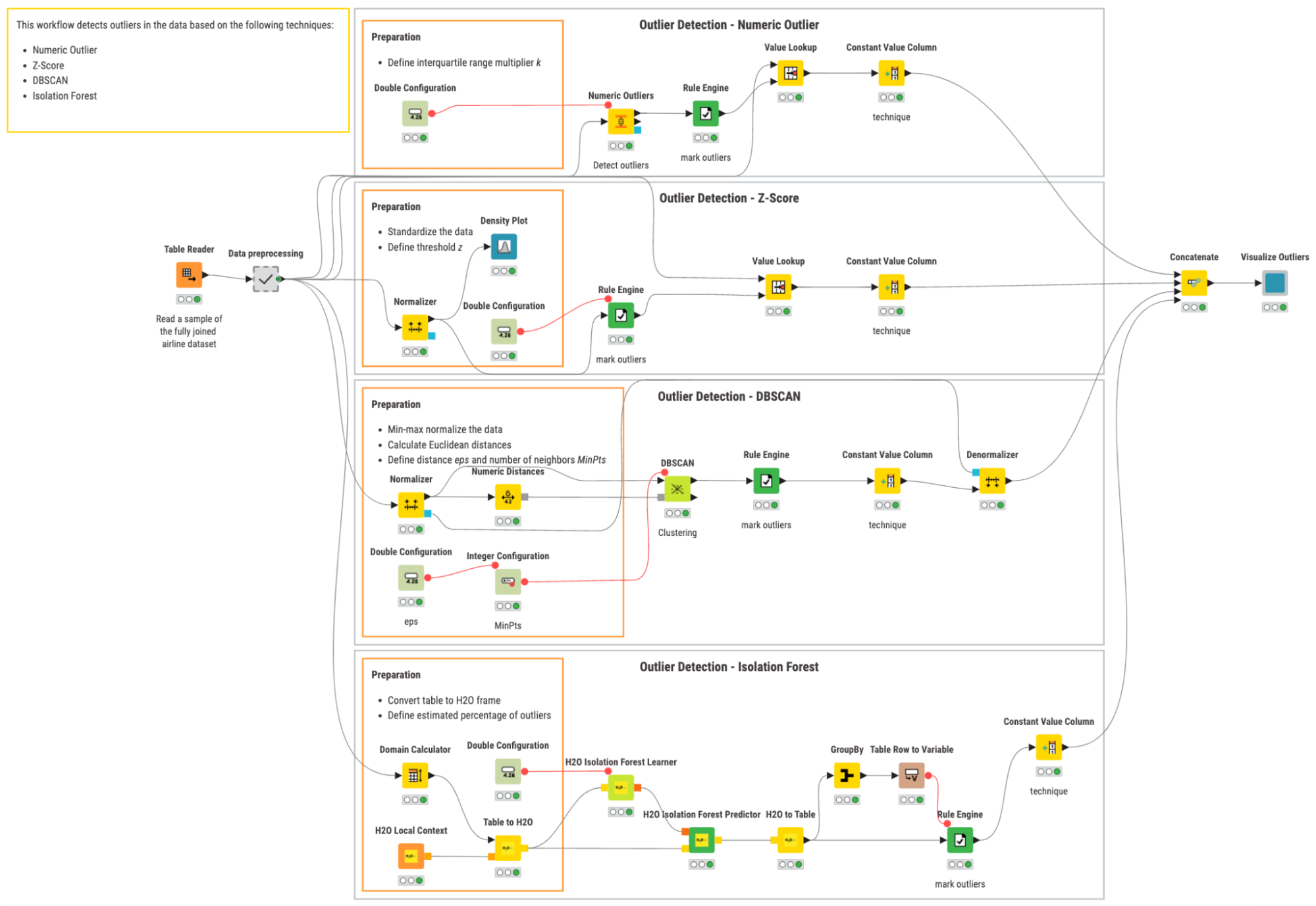
The KNIME workflow below implements the four proposed outlier detection techniques.

In the workflow, we:

1. Read the data sample with the Table Reader node
2. Preprocess the data and calculate the average arrival delay per airport inside the Data preprocessing metanode.
3. Detect outliers using the four selected techniques.
4. Compare the airports and techniques in a dashboard that the Visualize Outliers component produces using the Geospatial Analytics Extension for KNIME.

In the images below you can see the outlier airports as detected by the remaining three techniques. The results for the isolation forest technique are shown in Figure 1.

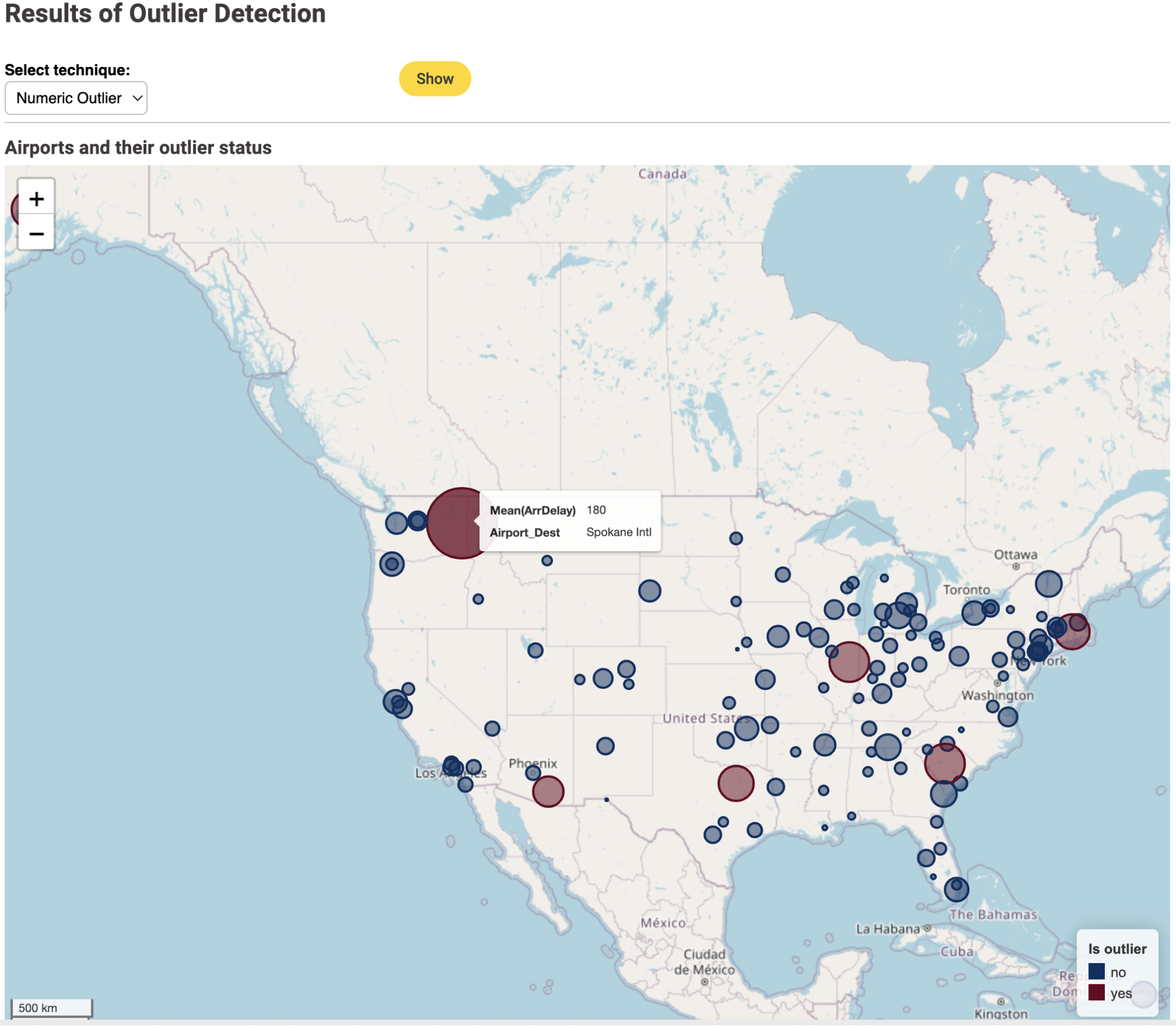
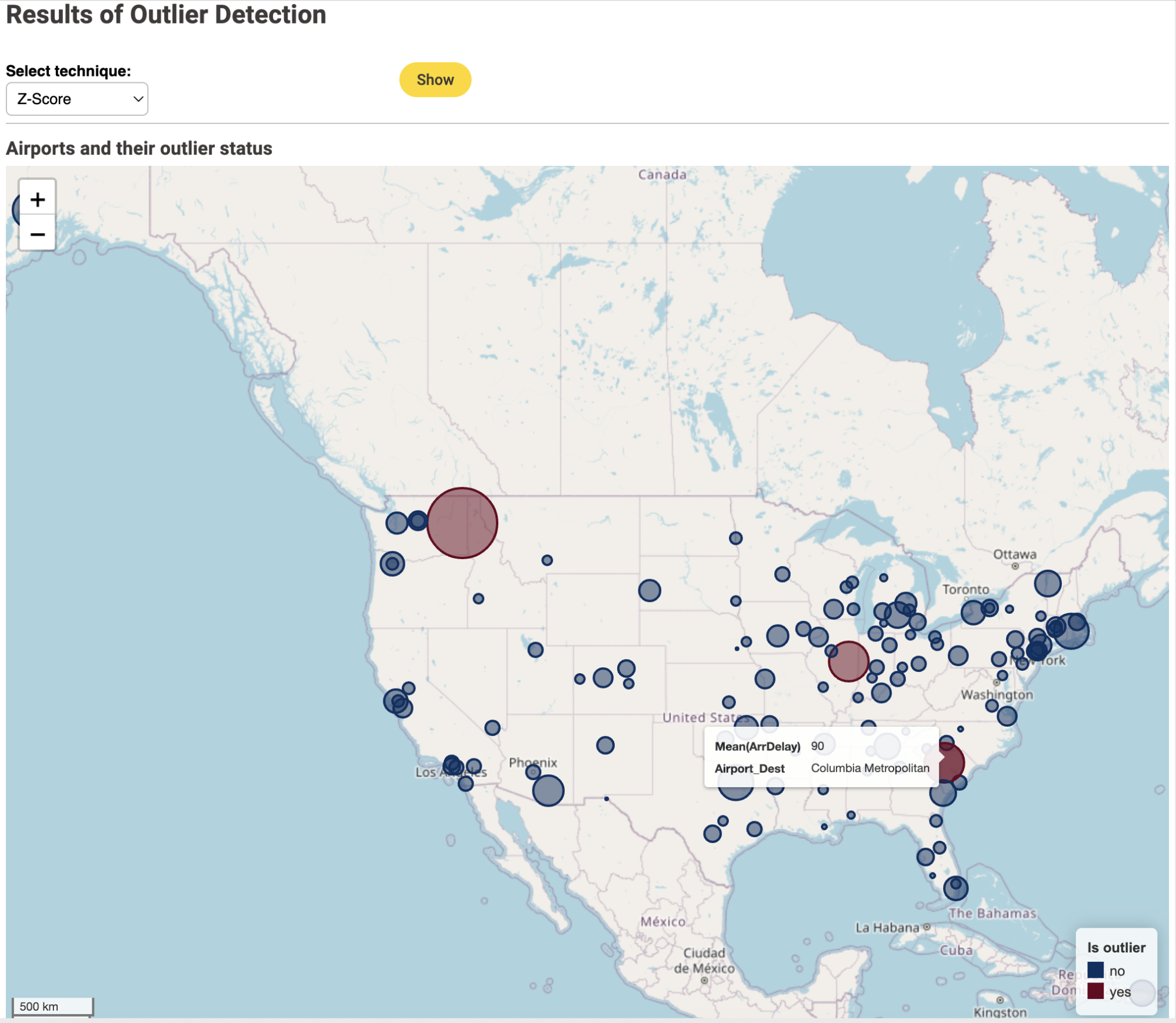
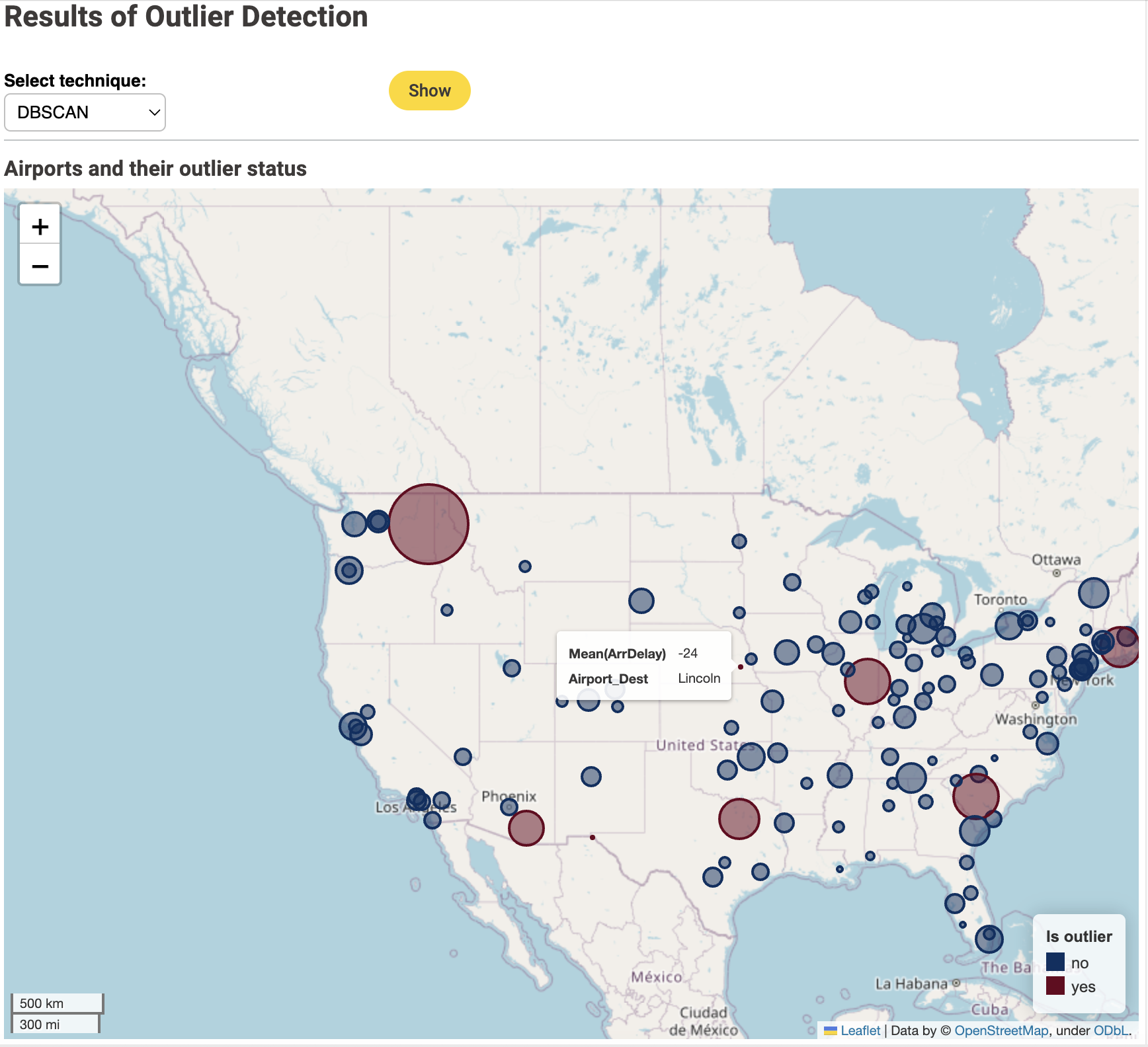
Similar to Figure 1, the blue circles represent airports with no outlier behavior while the red circles represent airports with outlier behavior. The average arrival delay time defines the size of the circles.

A few airports are consistently identified as outliers by all techniques: Spokane International Airport (Figure 3), University of Illinois Willard Airport and Columbia Metropolitan Airport (Figure 4). Spokane International Airport is the biggest outlier with a very large (180 min) average arrival delay. This airport could therefore be a candidate for further inspection of the airport processes and infrastructure.

A few other airports however are identified by only some of the techniques. For example Louis Armstrong New Orleans International Airport (Figure 1) has been spotted by only the isolation forest and DBSCAN techniques.

Note that for this particular problem the z-score technique identifies the lowest number (3) of outliers while the isolation forest technique identifies the highest number (13) of outlier airports.

Only the DBSCAN method (MinPts=15, ε=0.05, distance measure Euclidean) and the isolation forest technique (estimated percentage of outliers 10%) find outliers in the early arrival direction. You can find these outliers in Figures 1 and 5 as the red circles that are smaller than the blue circles.

Numeric Outlier

Z-Score

DBSCAN

In this blog post, we have described how to detect outliers and implemented four different outlier detection techniques in a one dimensional space: the average arrival delay for all US airports between 2007 and 2008 as described in the airline dataset.

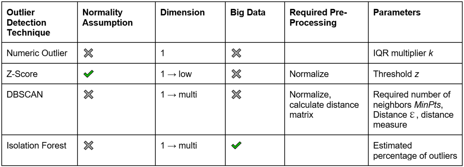
The four techniques we investigated are the numeric outlier, z-score, DBSCAN and isolation forest methods. Some of them work for one dimensional feature spaces, some for low dimensional spaces, and some extend to high dimensional spaces. Some of the outlier analysis techniques require normalization and a Gaussian distribution of the inspected dimension. Some require a distance measure, and some the calculation of mean and standard deviation. The characteristics are all summarized in Table 1.

There are three airports that all the outlier detection techniques identify as outliers due to the large average arrival delay.

However, only some of the techniques (DBSCAN and isolation forest) could identify the outliers in the left tail of the distribution, i.e. those airports where, on average, flights arrived earlier than their scheduled arrival time.

Authors: Maarit Widmann and Moritz Heine

References

• Download the workflow 07_Four_Techniques_Outlier_Detection from the KNIME Hub
• The theoretical basis for this blog post was taken from: Santoyo, Sergio. (2017, September 12). A Brief Overview of Outlier Detection Techniques [Blog post]