
What is Cohen’s kappa?
Cohen’s kappa is a statistical metric used in machine learning to score the performance of a classification model. It quantifies the agreement between two classifiers on categorical labels while correcting for the agreement that could occur by chance.
Put simply, Cohen’s kappa measures the agreement between two raters assessing the same thing. Sometimes, raters agree just by luck, so what makes Cohen’s kappa special is that it takes chance into account and corrects for that. This makes it particularly valuable when your data is imbalanced and one class heavily outweighs the other.
In this article, you’ll learn:
- When and why to use Cohen’s kappa, especially with imbalanced datasets
- How to calculate Cohen’s kappa
- Important pitfalls of Cohen’s kappa and how to avoid them
- How model balancing techniques (e.g. SMOTE) influence Cohen’s kappa
- How to evaluate models with the low-code tool, KNIME Analytics Platform
When to use Cohen’s kappa?
#1. When your data is imbalanced
In many real-word problems such as fraud detection, credit scoring, medical diagnosis, data can be imbalanced: One class (e.g. good credit) is much more frequent than the other (e.g. bad credit).
In these cases, overall accuracy becomes misleading because a model can be highly accurate simply by predicting the majority class.
How Cohen’s kappa helps: It adjusts the agreement that could occur simply due to the majority class, providing a more realistic estimate of the model’s performance.
Example: Imbalanced credit rating data
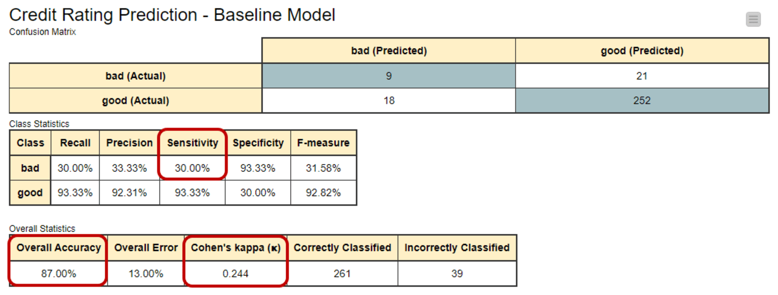
Using the German Credit Rating dataset, we artificially increased imbalance to 10% “bad” vs. 90% “good” credit ratings. A simple Decision Tree achieved:
- Accuracy of 87%
- Sensitivity (bad credit) of only 30%
- Cohen’s kappa: 0.244
The model looks accurate, but performs poorly on the minority class. Cohen’s kappa adjusts for this imbalance.
#2. When comparing human labels to model predictions
When training models in a supervised learning setup, we often treat human-labeled data as ground truth. Cohen’s kappa helps evaluate:
- The extent to which a model’s predictions agree with human labels
- How consistent human raters are with each other
#3. When you need a chance-corrected agreement metric
Unlike accuracy, Cohen’s kappa incorporates:
- Observed agreement
- Chance agreement (based on the distribution of predicted and actual classes)
Therefore, Cohen’s kappa can help evaluate more robustly whether an observed agreement exceeds what would be expected by chance given the label distributions.
How to interpret Cohen’s kappa in practice
Cohen’s kappa on imbalanced data
In the imbalanced credit rating example:
- The model correctly predicted most “good” customers.
- It missed most “bad” customers.
- Accuracy looked high, but Cohen’s kappa revealed the model’s inability to successfully predict the minority class.
To help us understand how well the model is doing beyond just accuracy, we look at Cohen's kappa value, which is 0.244 in this case. It's in a range from -1 to +1. The closer to +1, the better. So, 0.244 isn't great, indicating there's room for improvement in the model's performance.
Because Cohen’s kappa penalizes chance alignment with the dominant class, it exposes situations where the model is “cheating” by predicting the majority class.
You can see this in the confusion matrix and class/overall statistics for the baseline model. This is a Decision Tree model trained on our highly imbalanced training set. Here you can see the high overall accuracy (87%), although the model detects just a few of the customers with a bad credit rating (sensitivity just at 30%).
- Accuracy: 87%
- Sensitivity (bad credit): only 30%
- Cohen’s kappa: 0.244
Cohen’s kappa on balanced data
To improve the model’s performance, we can force it to acknowledge the existence of the minority class – the “bad” customers.
To do that, we train the same model on a training set where the minority class has been oversampled using the SMOTE technique.
This creates a more balanced dataset, with a 50/50 split between “good” and “bad” credit customers.
The improved model performs better on the minority class, correctly identifying 18 out of 30 customers with a “bad” credit rating. Cohen’s kappa for this improved model increases to 0.452. This is a significant improvement in agreement. Overall accuracy here is 89% – not so different from the previous value, 87%.
- Accuracy: 89% (almost unchanged)
- Cohen’s kappa: 0.452 (significant increase)
- Sensitivity for “bad” credit: 60%

This demonstrates that accuracy barely changed, but Cohen’s kappa nearly doubled. This reflects the model’s true improvement.
How to calculate Cohen’s kappa
Cohen’s kappa is defined as:
Where:
- p₀ = the observed agreement (“o” for observed), a.k.a. the overall accuracy, of the model
- pₑ = the expected agreement (“e” for expected) of the model, i.e., the agreement between the model predictions and the actual class values as if happening by chance
In a binary classification problem, like ours, pe is the sum of pe1, the probability of the predictions agreeing with actual values of class 1 (“good”) by chance, and pe2, the probability of the predictions agreeing with the actual values of class 2 (“bad”) by chance.
Assuming that the two classifiers - model predictions and actual class values - are independent, these probabilities, pe1 and pe2, are calculated by multiplying the proportion of the actual class and the proportion of the predicted class.
If we consider “bad” as the positive class, the baseline model (fig. 1) assigned 9% of the records (false positives plus true positives) to class “bad”, and 91% of the records (true negatives plus false negatives) to class “good”. Thus pe is:
Therefore, Cohen’s kappa statistics:
This is the same value you can see in the baseline model.
In simple terms, Cohen’s kappa helps us evaluate a classifier by considering how often it makes predictions that go beyond random chance.
Pitfalls of Cohen’s Kappa (and How To Avoid Them)
Cohen’s kappa is powerful, but it is not perfect. Below are the key pitfalls.
Pitfall #1. Cohen’s kappa’s range is theoretically [-1, 1], but not equally reachable
Why it happens
The maximum achievable Cohen’s kappa depends on how closely the predicted and actual class distributions match. When the model and the true labels assign classes in similar proportions, higher Cohen’s kappa values are easier to reach.
- If predicted and true class proportions differ significantly, the expected chance agreement increases. This lowers the maximum attainable κ.
- As a result, two models with identical accuracy can have different κ values simply because their predicted class proportions differ — making direct comparisons misleading.
How to avoid this pitfall
- Compare models on the same dataset, not across datasets with different class ratios.
- Inspect row/column totals in the confusion matrix.
- Consider processing the dataset carefully so class proportions are consistent when comparing models (e.g., balancing, stratified sampling)
See how this plays out in an example
In our baseline model (see the first table above), the distribution of the predicted classes closely follows the distribution of the target classes:
- 27 predicted as “bad” vs. 273 predicted as “good”
- 30 being actually “bad” vs. 270 being actually “good”.
For the improved model (see the second table above), the difference between the two class distributions is greater:
- 40 predicted as “bad” vs. 260 predicted as “good”
- 30 being actually “bad” vs. 270 being actually “good”.
As the formula for maximum Cohen’s kappa shows, the more the distributions of the predicted and actual target classes differ, the lower the maximum reachable Cohen’s kappa value is.
The maximum Cohen’s kappa value represents the edge case of either the number of false negatives or false positives in the confusion matrix being zero, i.e. all customers with a good credit rating, or alternatively all customers with a bad credit rating, are predicted correctly.
where pmax is the maximum reachable overall accuracy of the model given the distributions of the target and predicted classes:
For the baseline model, we get the following value for pmax:
Whereas for the improved model it is:
The maximum value of Cohen’s kappa is then for the baseline model:
For the improved model it is:
As the results show, the improved model with a greater difference in the distributions between the actual and predicted target classes can only reach a Cohen's kappa value as high as 0.853. Whereas the baseline model can reach the value 0.942, despite the worse performance.
Pitfall #2. Cohen’s kappa is higher for balanced data (even with the same model)
Why it happens
Kappa is maximized when the positive class probability is 0.5.That means that even a good model will get:
- Lower Cohen’s kappa on imbalanced test sets
- Higher Cohen’s kappa on balanced test sets
How to avoid this pitfall
- Always report the class distribution next to κ.
- When comparing models, test on datasets with consistent class ratios.
- Use balanced test sets during model development when possible.
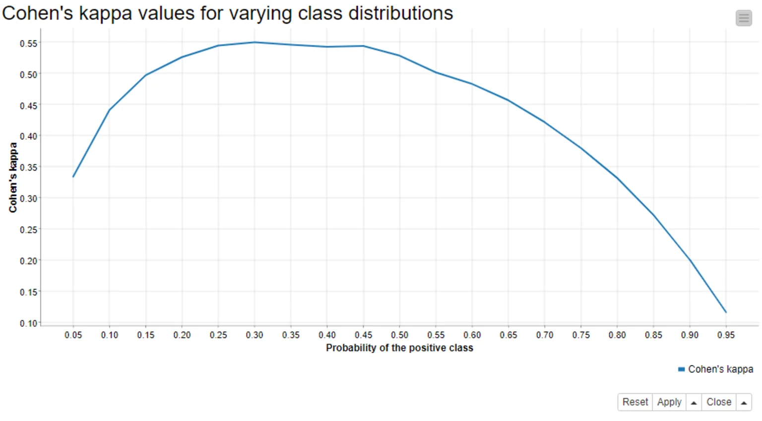
See how this plays out in an example
In experiments with multiple bootstrapped test sets, κ peaked when class proportions were equal — even though the model itself never changed.
When we calculate Cohen’s kappa, we strongly assume that the distributions of target and predicted classes are independent and that the target class doesn’t affect the probability of a correct prediction.
In our example this would mean that a credit customer with a good credit rating has an equal chance of getting a correct prediction as a credit customer with a bad credit rating.
However, since we know that our baseline model is biased towards the majority “good” class, this assumption is violated.
If this assumption were not violated, as in the improved model where the target classes are balanced, we could reach higher values of Cohen’s kappa.
Why is this? We can rewrite the formula of Cohen’s kappa as the function of the probability of the positive class, and the function reaches its maximum when the probability of the positive class is 0.5.
We test this by:
- applying the same improved model to different test sets, where the proportion of the positive “bad” class varies between 5% and 95%
- creating 100 different test sets per class distribution by bootstrapping the original test data, and
- calculating the average Cohen’s kappa value from the results
The graph below shows the average Cohen’s kappa values against the positive class probabilities – and yes! Cohen’s kappa does reach its maximum when the model is applied to the balanced data!
Pitfall #3. Cohen’s kappa says little about the expected prediction accuracy
Why it happens
κ measures agreement beyond chance — not the number of correct predictions.
For example:
- A model with accuracy = 87%
- Might have κ = 0.244, but that tells you nothing intuitive about “how many predictions will be right.”
How to avoid this pitfall
- Pair Cohen’s kappa with additional metrics:
- Accuracy
- Precision/Recall
- F1 Score
- Class-specific sensitivity
- Use κ to supplement—not replace—other performance indicators
See how this plays out in an example
The numerator of Cohen’s kappa, p0-pe, tells the difference between the observed overall accuracy of the model and the overall accuracy that can be obtained by chance. The denominator of the formula, 1-pe, tells the maximum value for this difference.
- For a good model, the observed difference and the maximum difference are close to each other, and Cohen’s kappa is close to 1.
- For a random model, the overall accuracy is all due to the random chance, the numerator is 0, and Cohen’s kappa is 0.
- Cohen’s kappa could also theoretically be negative. Then, the overall accuracy of the model would be even lower than what could have been obtained by a random guess.
Given the explanation above, Cohen’s kappa is not easy to interpret in terms of an expected accuracy, and it’s often not recommended to follow any verbal categories as interpretations.
For example, if you have 100 customers and a model with an overall accuracy of 87%, then you can expect to predict the credit rating correctly for 87 customers. Cohen’s kappa value 0.244 doesn’t provide you with an interpretation as easy as this.
Example KNIME Workflow: Cohen’s kappa for evaluating classification models
The workflow we used in this article was built with the open source KNIME Analytics Platform. KNIME Analytics Platform makes experimentation easy with its low-code, no-code interface — ideal for both beginners and advanced data scientists.
The workflow:
- Trains a baseline Decision Tree on imbalanced credit data
- Trains an improved version using SMOTE-balanced data
- Evaluates both models with accuracy and Cohen’s kappa
- Compares performance side by side
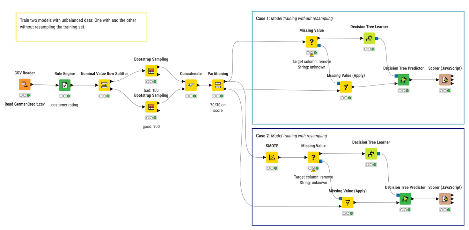
In the workflow we train, apply, and evaluate two Decision Tree models that predict the creditworthiness of credit customers.
- In the top branch, we train the baseline model
- In the bottom branch we train the model on the training set where the minority class has been oversampled using the SMOTE technique.