All you need is ... the Lag Column Node!

Time series prediction requires the prediction of a value at time t, x(t), given its past values, x(t-1), x(t-2), …, x(t-n). How do you implement a model for time series prediction in KNIME? For time series prediction, all you need is a Lag Column node!

For example, I have a time series of daily data x(t) and I want to use the past 3 days x(t-1), x(t-2), x(t-3) to predict the current value x(t). This is an auto-prediction problem. Introducing exogenous variables, like y(t) and z(t), into the prediction model, turns an auto-prediction problem into a multivariate prediction problem. Let’s stick with auto-prediction. What we will build is easily extendible to a multivariate prediction.

Time series prediction, then is just a data analytics problem with a particular input structure. In order to train a model for time series prediction, I need to create an input data table with the following structure: x(t-3) x(t-2) x(t-1) x(t). That is, I need to move the past 3 values of the time series in the same row with the current value x(t).

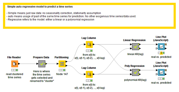
Once I have this structure, I can use for example a linear regression and model the target variable (current value) x(t) using its past 3 values x(t-3) x(t-2) x(t-1). It does not necessarily have to be a linear regression model: any supervised data analytics algorithm with numerical output will do.

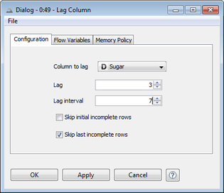
The Lag Column node has been introduced exactly to perform the first step, i.e. to move n past values of a time series onto the same row with the current value. You just need to specify the Lag (n=3 in this case) in the node configuration window, to move from row x(t) to row x(t-3) x(t-2) x(t-1) x(t).

This node can also put the current value and any past value side by side. For example, if I have daily data and I want to compare each value with the previous week value, I can set the Lag Interval to 7 in the configuration window and, after execution, I would get the following data rows: x(t-7) x(t). This is particularly useful for periodicity or seasonality correction.

After the Lag Column node has been applied (Lag=3), in our example, we used a Linear Regression Learner and Predictor respectively to train the model and to predict new values from the past.

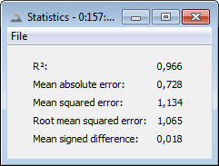
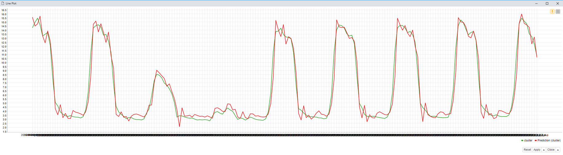
Finally, we apply the Numeric Scorer node on the newly predicted values to calculate the prediction error. The Numeric Scorer node calculates a few distance measures (R2, mean absolute error, mean squared error, mean root squared error, mean signed difference) between two time series, measuring then how big the error of our prediction is. The error View and the plot of the original time series vs. the predicted time series are shown respectively in figure 2 and 3.

In conclusion, you can run a time series analysis in KNIME with only three nodes: a Lag Column node to define the past, a Learner/Predictor node to build the model, and a Numeric Scorer to measure the prediction error.

The workflow used to implement a time series prediction (Fig. 4) is available on the EXAMPLES Server under Old Examples (2015 and before) 001_TimeSeries.

A more complete example on how to build a workflow for time series analysis is also available here on the KNIME Hub.