
As part of the KNIME Student Challenges program, KNIME co-organizes student challenges with educational institutions with the aim to connect with professors around the globe to create low-code challenges for their students.
One of the recent submissions came from ISCTE Business School in Lisbon, Portugal. Together with Patrícia Filipe, Associate Professor at ISCTE Business School, the students in her class were challenged on the topic of fraud detections.
Marta Couto is one of the winners of this KNIME Students Challenge and completed a 3-month internship at KNIME in Konstanz. This blog post is the result of one of the projects she worked on during that time.
The sports betting market has experienced exponential growth in recent years, largely driven by easy access to digital betting platforms. It is estimated that the global value of this market has surpassed 100 billion dollars annually, with projections indicating continued growth through the end of the decade. This expansion has, in parallel, fueled the development of sports analytics, with professional bettors and betting operators increasingly relying on analytical models to predict outcomes, identify gameplay patterns, and calculate more precise and highly accurate probabilities.
However, despite the highly sophisticated analytical models employed by betting companies, soccer, like all sports, remains deeply unpredictable. And therein lies the true beauty of sport. No matter how much data is analyzed, there is always room for the unexpected: A goal in extra time, an improbable save, a penalty that changes everything.
In this article we will analyze such moments in the most recent Bundesliga season (2024/2025). Based on data provided by betting offices indicating the odds for each game and team, the following has been observed:
- What factors may have contributed to the occurrence of the least likely outcomes in these matches (the so-called upsets)?
- Why did the game not unfold as predicted by the betting markets?
Soccer in numbers: Betting odds and market values
Betting market predictions & match statistics
To carry out this analysis, we used a dataset which provides match statistics as well as betting market predictions for each game. The dataset contains 206 rows, each representing a match from the 2024/2025 Bundesliga season. We have manually removed the Union Berlin vs. Bochum match on December 14, 2024. In this special case, the game was interrupted due to violent incidents during the match and was later decided to award Bochum a 2:0 win, as the official website of the Bundesliga states.
For each game, the dataset includes statistical indicators such as the number of shots taken by each team, shots on target, yellow and red cards received, corners, fouls, halftime result, and full-time result, amounting to a total of 20 columns. All columns are numeric, except the following columns:
- “Date” and “Time”, indicating each match’s date and start time.
- “AwayTeam” and “HomeTeam” each indicating which teams played against each other.
- “HalfTimeResult” and “FullTimeResult” each indicating the match result after the first half and after the second half respectively (“H”: home team winning; “A”: away team winning; “D”: draw).
In addition, the dataset provides detailed information on betting odds from various bookmakers, including both maximum and average odds for home win, draw, and away win outcomes, as well as odds for the goals market (>2.5 and <2.5) and Asian handicap (a betting system originated in Asia in which teams are handicapped according to their form).
Market value of teams
Another key factor in explaining unexpected results could be the market value of the starting line-ups. Beyond helping to quantify the theoretical gap between teams, it also reflects their actual strength at the time of the game which often differs from the squad’s overall valuation. Factors such as injuries, suspensions, player rotation, or tactical choices can significantly alter the quality of the eleven players on the pitch. By incorporating this variable, we aim to better understand whether upsets (i.e. the occurrence of the least likely outcome in a match) are more likely to occur when a favorite fields a weakened side, or when an underdog lines up its best assets.
Unfortunately, we could not find a public dataset that reflects the market values of the teams, hence, we decided to use web scraping to collect the desired information from a sport statistics website. In KNIME, web scraping can be done using the nodes of the KNIME Web Interaction (Labs) extension. This workflow is available for download from the KNIME Community Hub. In our case, we implemented the data collection process in three steps:
Step 1: First, we compiled a list of all URLs needed. In total, the Bundesliga season has 34 match days with 9 games played each match day. Hence, we collected a total of 306 URLs where each URL redirects to the match-individual statistics, including the total market value of the squad.
Step 2: In the second step, we accessed each URL and collected the desired value (total market value of the starting line-up as well as substitutes for both home and away team).
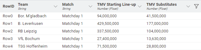
Step 3: Once all data was collected, all that was left to do was to perform some data wrangling to get the scraped data into a structured data format. The result is a dataset (see Figure 1) containing the market values of all teams for both their starting line-up (“TMV Starting Line-up”) as well as substitutes (“TMV Substitutes”) - one value for each match day.
Logistic Regression for identifying influencing factors
Data pre-processing
Before merging both datasets, it was necessary to carry out some data cleaning and transformation, particularly through the creation of new columns.
First, we began by converting the odds into probabilities, since:
- Probabilities are better suited for analytical modeling. As probabilities usually range on a normalized scale between 0 and 1, it allows for consistent interpretation and comparison. Odds on the other hand do not follow a standardized total across scenarios and can vary infinitely.
- It is easier to interpret probabilities. It is more intuitive to say that a team has a 20% chance of winning a match according to the betting odds than to say the odds are 5.1.
- Probabilities allow direct comparisons between games and teams. For example, it is accurate to say that if one team has a 20% chance of winning and the other 40%, then one has twice the chance of the other. With odds like 2.5 and 5.0, that interpretation would not be valid since odds do not scale linearly with probabilities. While odds of 2.5 correspond to a 40% chance and odds of 5.0 to a 20% chance, the numerical ratio between the odds (2.5 vs. 5.0) does not reflect the ratio between the underlying probabilities.
Below in Figure 2 we see an abstract of the odds as provided in the dataset. Let’s have a closer look at the five columns and what they mean:
- AvgHomeOdds: The average odds that the home team will win.
- AvgDrawOdds: The average odds for a draw.
- AvgAwayOdds: The average odds that the away team will win.
- Avg>2.5: The average odds that there will be 3 or more goals scored in the match.
- Avg<2.5: The average odds that there will be a maximum of three goals scored in the match.
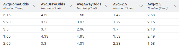
Looking at the first data row in Figure 2 indicates that the odds for the home team winning is 5.16 (AvgHomeOdds), the odds for the away team winning is 1.58 (AvgAwayOdds), and the odds for a draw is 4.53 (AvgDrawOdds). Now, if you would bet 1€ on the home team winning, your bet is multiplied by the factor 5.16. Hence, if the home team wins (i..e, you win your bet), you would win 1€ * 5.16 = 5.16€. The other way around, if you would bet on the away team winning, you would only win 1€ * 1.58 = 1.58€.
This means the more likely an event, the less money you will win and vice versa. So, by looking at the odds, we are able to understand that in this scenario, the home team winning is much less likely compared to the away team winning, hence, the higher odds for the home team winning. However, it is not clearly understandable how much the probabilities of home team winning vs. away team winning actually is.
Therefore, let’s have a look at Figure 3 below. Here, it shows the probabilities of the different scenarios after converting from odds into probabilities - which makes interpretation much easier. Similar as before, the first three columns give us the probabilities that the home team wins (“ProbHome”), that the match results in a draw (“ProbDraw”), or that the away team wins (“ProbAway”). Looking at the same match in the first row, it is now much easier to understand that the away team has a much higher chance of winning (0.633 or 63.3%) than the home team (0.194 or 19.4%).
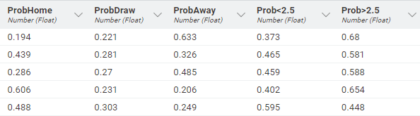
To convert betting odds into implied probabilities, the following formula is applied:
Prob = 1/Odds
Note: The sum of the implied probabilities for home team winning, away team winning, and draw (ProbHome+ProbAway+ProbDraw) exceeds 100. This is because of the bookmaker’s margin (i.e., their built-in profit.). This can be adjusted by dividing each probability by the total.
Next, we created the columns “Underdog” and “Favorite” using the Expression node. The “Underdog” column identifies the least likely outcome in each match (“A”: away win; “D”: draw; “H”: home win), while the “Favorite” column indicates which team is favored by the odds (“H”: home team is favored; “A”: away team is favored).
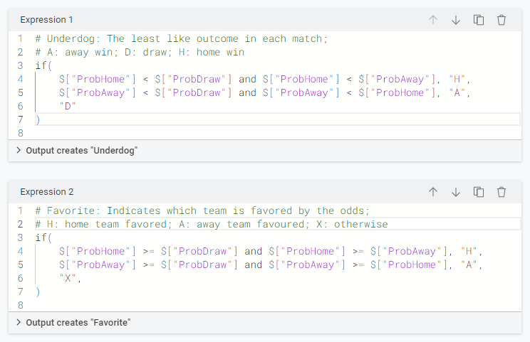
It is worth noting that, in 46.89% of the matches, a draw (“D”) was the least likely outcome, and in 67.87% of the matches, the home team was considered the favorite to win.
Feature Engineering
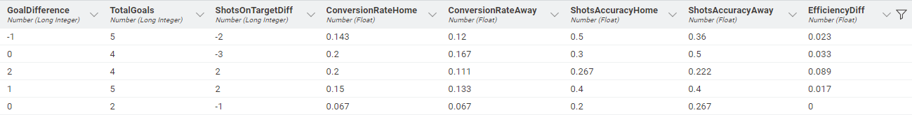
To extract some initial statistical insights, we created eight additional columns related to offensive performance:
- “GoalDifference”: The final goal difference between the teams.
- “TotalGoals”: The total goals scored in the match (sum of both teams’ goals).
- “ShotsOnTargetDiff”: The difference in shots on target between the two teams.
- “ConversionRateHome”: The percentage of shots by the home team that resulted in a goal.
- “ConversionRateAway”: The percentage of shots by the away team that resulted in a goal.
- “ShotsAccuracyHome”: The percentage of shots by the home team that were on target.
- “ShotsAccuracyAway”: The percentage of shots by the away team that were on target.
- “EfficiencyDiff”: A measure to compare offensive efficiency.
Using the GroupBy node, we were able to identify the teams with the strongest offensive performances. We found that FC Bayern München had the most total shots (640) during the 2024/2025 season, while Holstein Kiel had the fewest (367). Regarding shots on target, Bayern München again led with 269, while FC St. Pauli had the lowest (114). As for conversion rate per team (percentage of shots resulting in goals), Bayer Leverkusen led with a 17.2% rate, while VfL Bochum had the lowest, at only 7.8%. The component “Offensive Performance” visualizes these findings.
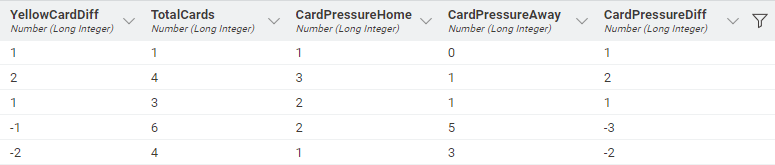
Considering that discipline and cards can significantly influence match outcomes, we created 5 more columns:
- “YellowCardDiff”: The difference in yellow cards between the teams.
- “TotalCards”: The total number of yellow and red cards in the match.
- “CardPressureHome”: A measure for the disciplinary load of the home team.
- “CardPressureAway”: A measure for the disciplinary load of the away team.
- “CardPressureDiff”: A measure to compare disciplinary pressure.
This analysis revealed that FC Augsburg and Holstein Kiel were the most undisciplined teams, each receiving 77 yellow cards over the season, while FC Bayern München received the fewest (48). Additionally, Borussia Dortmund had the highest number of red cards (6).
We also considered it relevant to include the column “Turnaround”, which captures matches where the result changed between half-time and full-time, i.e., one team was winning at the break but the other ended up winning the match. Out of the 305 matches analyzed, this happened in only 15 cases (4.92%). Leipzig was involved in the highest number of such matches (6), losing 4 and winning 2. Stuttgart, on the other hand, was the team that managed to successfully turn the score in their favor most often (3 times).
We then arrive at the core of this article, the creation of the “Upsets” column which labels with “1” the matches whose outcomes were the least likely according to betting odds. Out of 305 matches, 67 (21.97%) ended in unexpected results.
The next step involved merging the two datasets (Betting Market Predictions and Market Value) using the Joiner node. After some data processing, we were able to incorporate the market value of the starting lineup for each team in every match. As a point of interest, the most valuable starting lineup this Bundesliga season belonged to Bayern Munich, with a total market value of €609,000,000, while the least valuable was from Holstein Kiel, with €13,450,000 (note that market values change throughout the season).
Having the market value per team for each match allowed us to pose the question: Is the team with the higher market value also the favorite to win, according to the odds? To address this, we created the “Market_vs_Favorite” column which assigns “1” when the more valuable team is also the one favored by the odds and “0” otherwise. Looking at the column shows that in ca. 80% of matches the more valuable team is also the one favored by the odds.
As the final step in the exploratory data analysis, we created the “DiffProbAH” column, which represents the difference in win probability between the two teams. The match with the greatest predicted gap was between Bayern Munich and Holstein Kiel, with a probability difference of 92.6% in favor of Bayern. Conversely, matches such as Werder Bremen vs. Freiburg and Mönchengladbach vs. Frankfurt had equal win probabilities for both teams (DiffProbAH = 0).
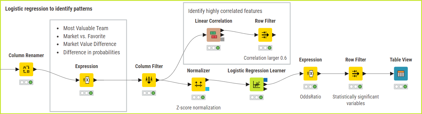
Exploratory data analysis with logistic regression
With the data processing complete and variables normalized, we proceeded with a logistic regression analysis (see Figure 7).
Our aim is to understand which factors influence the likelihood of unexpected results (target = “Upsets”). Outlined below are the variables incorporated into the analysis:

Figure 8. The features included in logistic regression analysis.
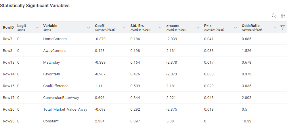
After running the logistic regression using the Logistic Regression Learner node, we identified seven statistically significant variables (p < 0.05) that influence the probability of an upset:
- HomeCorners: Each additional corner by the home team is associated with 31.5% lower odds of an upset. This suggests that the more offensively dominant the home team (typically the favorite) is, the lower the chances of a surprising outcome.
- AwayCorners: Each additional corner by the away team leads to a 52.6% increase in the probability of an upset. This may indicate that the underdog is creating offensive opportunities, signaling a potential to surprise.
- Matchday: For each progressing matchday (e.g., from Matchday 10 to 11), the probability of an upset decreases by 32.3%. This could reflect that as the season advances, favorites tend to stabilize their performance, making surprises less frequent.
- Favorite=H: When the home team is the favorite to win, the chances of an upset decrease by 62.7%. This confirms previous findings regarding the advantages of home favorites.
- GoalDifference: Each one-unit increase in goal difference in favor of the underdog triples the likelihood of an upset (OddsRatio = 3.025). A decisive victory by a non-favorite is a strong indicator of a surprising result.
- ConversionRateAway: A higher finishing efficiency by the away team doubles the probability of an upset (OddsRatio = 2.005). In other words, efficient underdogs become particularly dangerous.
- Total_Market_Value_Away: The greater the market value of the away team, the lower the chance of an upset. In this case, the probability drops by 50% per one-unit increase. This may indicate that the away team is not a true underdog when its market value is high.
Looking Ahead: Key Takeaways
All things considered, although football events are often random and unpredictable, there are some factors that can help explain the occurrence of surprising results – even though any true football fan enjoys unexpected and improbable outcomes!
The final workflow is shown in Figure 10 and is available for download from the KNIME Community Hub.
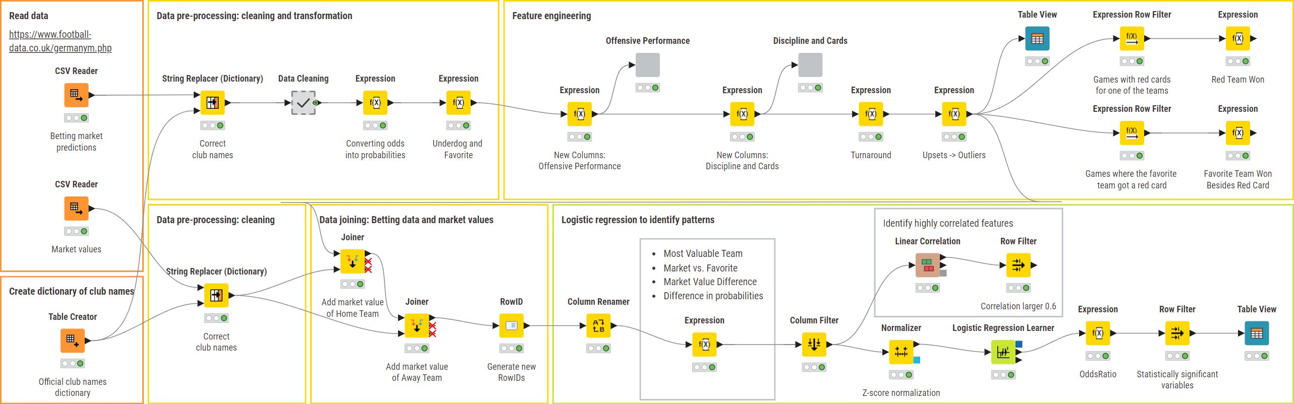
In conclusion, we highlight some recommendations for ways to deepen the analysis in future studies, namely:
- Include temporal and contextual factors: incorporate recent team form, previous result streaks, the presence of injuries, suspensions or coaching changes, and the importance of the match;
- Test predictive models that capture non-linearities or complex interactions: decision trees, random forests, and gradient boosting.