Linear programming is a widely used mathematical approach to optimizing outcomes under a set of constraints. It is applied in areas such as planning, logistics, technology, and more.
A logistics manager aiming to reduce the cost of truck shipping. For this, they must consider multiple constraints, such as weight limits, on-time delivery requirements, or choosing which products to include based on value, size, and weight. While these problems may seem complex, they can be solved efficiently with linear programming.
The Optimization component in KNIME integrates linear programming directly into KNIME workflows, making it accessible so you can model and solve optimization problems without requiring advanced mathematical expertise. You can easily set constraints and calculate optimal solutions, simplifying decision-making for a variety of tasks. This component is built on the SciPy optimization library, a widely used and well-documented Python toolkit, available here.
Whether you’re managing a departmental budget or building a fantasy football team under strict rules, this component provides a straightforward solution.
Use Case: Minimizing the number of trucks
To show how KNIME’s Optimization component works in practice, we’ll walk through a classic linear programming scenario: loading items into trucks while minimizing the total number of trucks used.
In this example, let’s say we are managing a warehouse filled with various items. Each item has specific weights, volumes, and available quantities. The goal is to assign these items to as few trucks as possible while ensuring each truck remains within the following constraints:
- Maximum Number of Items: Each truck can carry up to 10 items.
- Weight Limit: The total weight of items must not exceed 175 lbs per truck.
- Volume Constraint: The combined volume of items must stay within 2000 m³ per truck.
Problem setup
Each item in the shipment is defined by the following attributes:
- Weight (lbs): The weight of a single item.
- Volume (m³): The space occupied by a single item.
- Count: The number of units available for shipment for each item type.
The goal is to assign items to the fewest number of trucks as possible while staying within the defined limits for weight, volume, and item count.
In the next step, we’ll translate this real-world scenario into a format suitable for KNIME’s Optimization component.
Setting up Your KNIME workflow
This truck-loading example focuses on minimizing the number of trucks while ensuring that each one stays within defined limits for item count, weight, and volume.
To achieve this, we implement a recursive loop, where each iteration corresponds to one truck. At each step, the task is to decide whether an item should be included in that truck’s load. Since every item has a quantity of one, the decision is binary: include or exclude.
Before the Optimization component can be used, the input data must first be converted into the required format.
Variables table:
- Each item is treated as a variable and given equal priority.
- To maximize the number of items selected for a truck, each item is given an objective function weight of –1. This is because KNIME’s Optimization component performs minimization by default, so maximization problems are handled by minimizing the negative of the objective.
- The lower and the upper bounds are set to 0 and 1, representing a binary decision: include the item or not
- The “Integer” column is set to True because items cannot be split, this turns the problem into a Mixed-Integer Linear Programming (MILP) scenario.
Constraints table:
- Each item is represented as a column, with its corresponding count, weight, and volume data.
- The constraint values (e.g., truck weight limit, volume limit, and item capacity) are provided as a column.
- The “Equals?” column is set to False, indicating that the constraints allow flexibility: values must stay within the defined limits, but they don’t have to match them exactly.
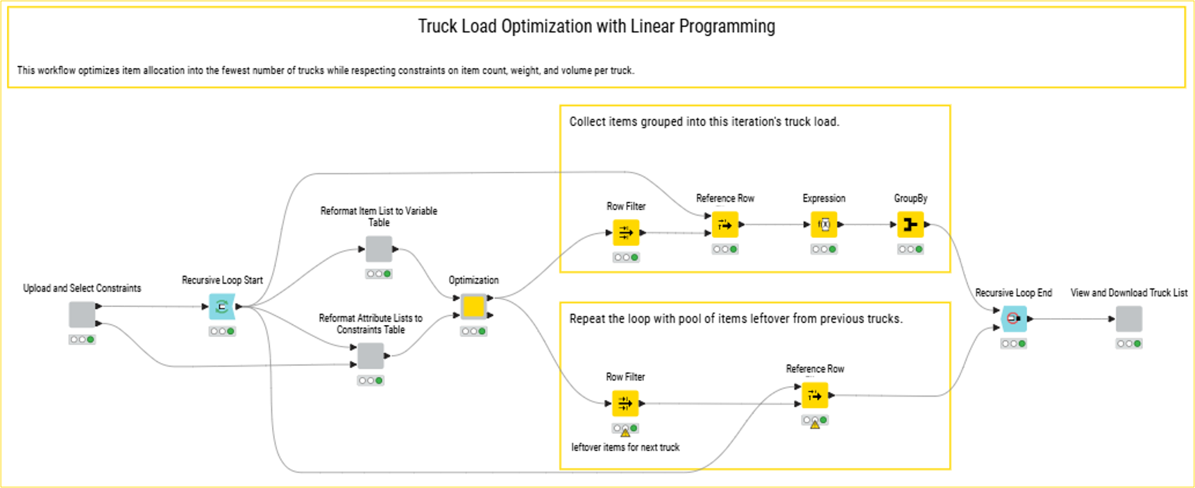
Visualize and scale your results
The output of the optimization component is processed in two parts. First, it captures data for the current truck, including the items selected, their count, total weight, and volume. This information is later used to visualize the solution.
Second, the selected items are removed from the full list, and the remaining items are returned as input to the recursive loop. This loop continues until all items are assigned to trucks. Through this iterative process, the number of trucks is minimized while adhering to the defined constraints.
To understand the result, we can visualize how items were allocated across trucks. In the scatter plot below, each point represents a truck. The x-axis shows the total weight and the y-axis shows the total volume.
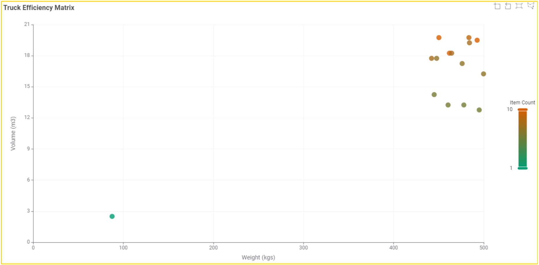
Most trucks appear on the right top corner of the scatter plot, indicating near-full capacity. One outlier in the bottom left corner represents the last truck, which contains only a single item that couldn’t fit in the earlier trucks. While further optimization like redistributing weights might improve efficiency, the goal here is to demonstrate a valid linear programming solution under multiple constraints.
Once the optimization is complete, you can export or save the file containing the optimized truck allocation, which includes the list of items assigned to each truck, ready for use in your specific use case.
Solving logistics problems with KNIME
Optimization problems like this one are common in many industries, from logistics and supply chain management to finance, manufacturing, and scheduling. The approach demonstrated here can be applied to a wide range of scenarios where decisions must be made under constraints.
In this blog post, we demonstrated how to solve a real-world logistics problem using KNIME’s Optimization component. The use case focused on minimizing the number of trucks required to ship a set of items while staying within defined limits for weight, volume, and item count. We showed how to prepare the data, configure the Optimization component, and visualize the results, all within a KNIME workflow.