
Analyzing a population requires a representative sample of it that reflects the characteristics of the population. Otherwise the analysis of the sample won’t generalize to the population. At the same time, a carefully designed sample is enough to reveal the patterns and characteristics of the whole population, should that population be unreachable as a whole, too expensive to collect, or is evolving quickly.
On the other hand, we can also capitalize on statistical sampling methods to tackle the problem of the lack of rare examples and thus uneven data representation, which affects the performance and generalizability of machine learning models.
To ensure that our samples are representative and maximize the performance of a machine learning algorithm, in this article we want to:
- Explain some of the most popular statistical sampling techniques
- Walk through a use case that highlights the effect of a sample design to model performance
- Point you to a workflow that illustrates how some of these sampling strategies can be carried out in KNIME.
Note. The workflow used throughout this article is freely available on the KNIME Hub if you would like to play with the data or experiment with different strategies by yourself.
Five Designs for Samples to Represent Your Population
Let’s first tackle the issue of designing a random sample that represents your population the best. We will introduce the following strategies, and give examples on which type of population they work the best for:
- Random sampling
- Stratified sampling
- Cluster sampling
- Linear sampling
- Take from the top
Random sampling
You could say that simple random sampling is a bit like a lottery where we are randomly selecting a number from a box. For data scientists, it means we are randomly picking a data point from our dataset.
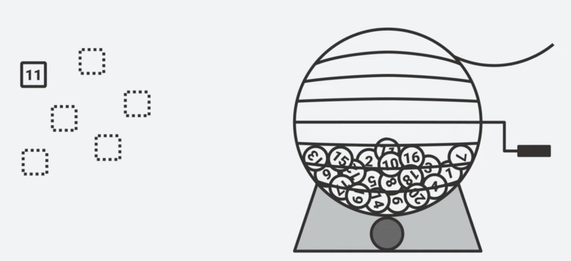
Put more technically, in simple random sampling we don’t introduce any bias to how we select a sample from the population. Every possible sample of a given size has the same chance of selection.
While simple random sampling is praised for its simplicity and lack of bias, it doesn’t guarantee the presence of all types of samples nor does it preserve the order of the data. If this is what you need, then we can use one of the sampling strategies below.
Stratified sampling
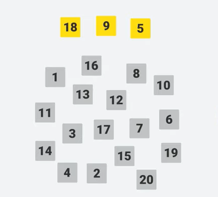
In stratified sampling, we consider that a feature partitions a heterogeneous population into homogeneous subgroups - called strata - and that our analysis will vary among the different subgroups. With stratified random sampling we can ensure that representatives of all subgroups are included in the sample.
In a sample extracted by stratified sampling, the distribution of the strata will be the same as in the population. For example, let’s say we randomly select 5 players from a pool of 3 goalkeepers (yellow in Figure 2) and 17 outfield players (gray in Figure 2). If we did this via stratified sampling, then we will likely have 3⁄20*5 ≈ 1 goalkeeper and 17⁄20*5 ≈ 4 outfield players - which sounds like a reasonable team!
Stratified random sampling provides an unbiased and accurate representation of the a priori distribution of a feature in an underlying population. However, it can only preserve the distribution of a nominal feature. Otherwise we need to rely on other sampling strategies, such as cluster sampling.
Cluster sampling
Cluster sampling partitions the data into clusters that share similar characteristics such as latitude and longitude. It then samples whole clusters randomly from the population. All the members from these randomly selected clusters constitute the final sample.
If that sounds the same as stratified sampling, the difference between stratified and cluster sampling is that in stratified sampling we identify groups and then randomly sample from those groups. In cluster sampling, we identify groups and use some of those groups as our sample. In cluster sampling the groups can also overlap.
For example, suppose you want to investigate how well your product would do in a new country, let’s say Japan. Instead of performing stratified sampling for each town in Japan, we would carry out cluster sampling by identifying cities and then carrying out an experiment only in certain cities, but not all of them. This makes the sampling process much more efficient!
But cluster sampling has some drawbacks. The most important one is its reliance on the design of each cluster. The quality of the clusters and how accurately the sampled clusters represent the underlying population heavily determine the validity of our results. In practice, clusters often yield a partial representation of the population’s characteristics, as they tend to be more internally homogeneous than the population as a whole, hence potentially leaving out essential characteristics.
Last, we introduce two simple sampling techniques, linear sampling and take from the top.
Linear sampling
Linear sampling extracts a data point every n samples, for example, every 10th observation in the population. This sampling strategy is a simple way of extracting a sample that contains all types of data from the population, yet it only works if the data doesn’t show any pattern at regular intervals. This is often the case in time series data, for which you can then use the take from the top strategy, which we introduce next.
Take from top
The Take from top sampling strategy preserves a sample from the population as a chunk from the top. This strategy is used for time series data, where the time order of observations in the population needs to be preserved in the extracted sample. Furthermore, when partitioning data for a time series model, this strategy ensures that the model is trained on past data (at the top) and tested on future data (at the bottom). However, this strategy doesn’t guarantee that the data represents the entire population and shouldn’t be used when the goal is to extract a random sample.
These statistical sampling techniques are formidable allies to constitute a representative sample of our population, but they can also tackle, for example, the problem of imbalanced datasets.
Two Designs for Sampling Imbalanced Datasets
Here we tackle the second issue with random sampling - imbalanced data. Imbalanced datasets pose a problem of representation, in that one group - the minority class - contains significantly fewer samples than the other group - the majority class. Class imbalance is especially detrimental to the construction of generalizable machine learning models as they learn to predict the majority class accurately but fail to capture the minority class. If adding new data is not a feasible option, to balance uneven datasets, we can use two sampling techniques: undersampling or oversampling.
- Undersampling works by keeping all of the data in the minority class and decreasing the size of the data in the majority class to equal the size of the minority class. The most remarkable disadvantage of undersampling is the loss of potentially important information for the training of models, since data is removed without any consideration of what it is or how meaningful it might be for analysis.
- Oversampling, on the other hand, solves the problem of imbalanced datasets by increasing the number of data points in the minority class to equal the size of the majority class.
We introduce two popular techniques for under- or oversampling called bootstrapping and synthetic minority oversampling technique (SMOTE).
Bootstrapping
This is simple random sampling but administered with replacement, that is, once a datapoint is picked it goes back into the population and thus may be chosen more than once. This technique can create duplicates of the data points in the minority class and also discard some representatives of the minority class.
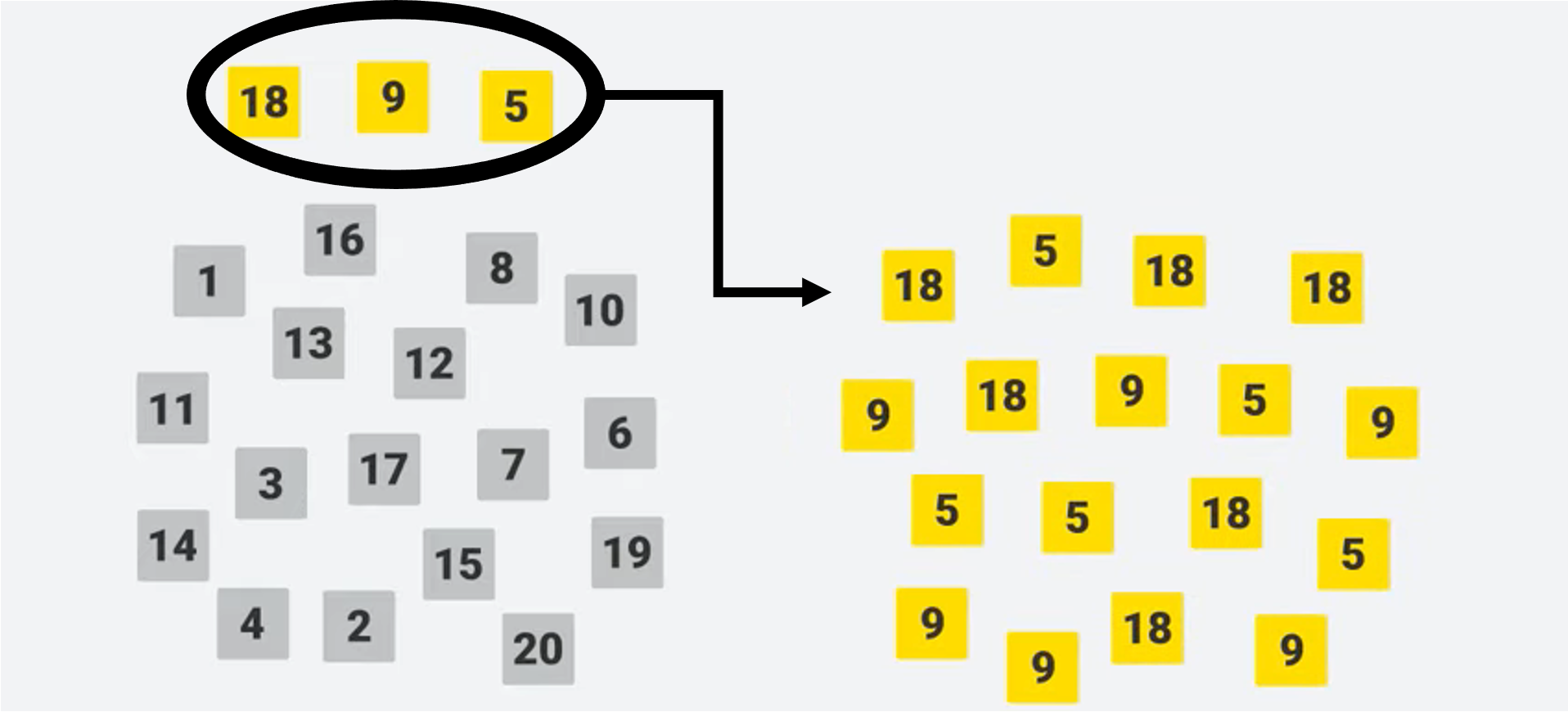
The figure above shows a population with imbalance classes grey/yellow on the left. On the right is a bootstrap sample of the minority class (yellow), which contains duplicates due to the replacement.
Synthetic Minority Oversampling Technique (SMOTE)
This works by randomly picking a data point from the minority class and one of its k-nearest neighbors within the minority class. The synthetically generated data point lies then at a random point on the vector connecting these two data points in the feature space. It is worth mentioning that this technique does not create duplicates.
While oversampling techniques have the clear advantage of not losing potentially important information in our majority class, they can be computationally expensive and slow down the speed of our analysis.
Learn more about oversampling:
SMOTE: Synthetic Minority Over-sampling Technique
Data Science Pronto! Bootstrapping - KNIMETV, YouTube
Now that we have talked about the uses for different sampling strategies, let’s try out these techniques on a healthcare dataset on Kaggle for predicting stroke events.
Example Workflow: Experiment with Statistical Sampling
We’ve built a workflow that you can use to experiment with simple random sampling and stratified random sampling (Partitioning node), undersampling (Equal Size Sampling node) and oversampling (Bootstrap Sampling node and SMOTE node).
The workflow draws on the kaggle Stroke Prediction Dataset which represents 5110 rows with 11 clinical features such as body mass index, smoking status, age, gender, and glucose level. The task is to predict stroke (yes/no), which is a classification problem. We chose to build a Random Forest model in KNIME.
The data is highly imbalanced as you can see in the Figure 4 generated by the Data Explorer node. The histogram shows that most of the people (over 90%) have not had a stroke.
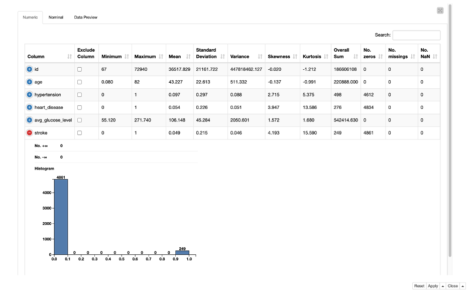
Trivia: “Imbalanced data” is a term generally reserved for 90% or more of one class and 10% or less of another class, but that is a guideline – not a rule. In extreme cases like fraud detection, fraudulent transactions may constitute less than 1% of the data.
Introducing the workflow
The workflow in Figure 5 experiments with different sampling strategies of the training and test sets (aka partitioning) and with different strategies to handle class imbalance in the training data (aka resampling). Finally, it compares their performances in the stroke prediction.
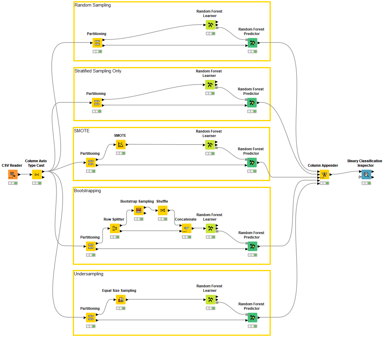
The workflow implements random partitioning as the baseline at the top and stratified partitioning for the remaining models. Below we point to the nodes that implement the different sampling strategies:
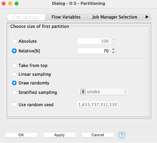
- The Partitioning node creates the training and test sets via the options for random, stratified, linear and take from top in its configuration dialog:
- The SMOTE node performs oversampling of the minority class on the training data. It allows us to choose the number of nearest neighbors, as well as whether to oversample the minority class only or to oversample each class equally.
- The Equal Size Sampling node performs undersampling of the majority class by randomly discarding majority class data.
- The Bootstrap Sampling node allows for bootstrap sampling to obtain a certain sample size defined as % of the input data or as the absolute sample size. Additionally, we have the option to append the count of occurrences to track the number of duplicate rows for each originally unique data point.
Finally, we want to check how much we can improve the model’s performance by selecting the most appropriate sampling method.
Compare Statistical Sampling Strategy Results
We can evaluate the models’ performances and interactively inspect the results by taking advantage of the Binary Classification Inspector node.
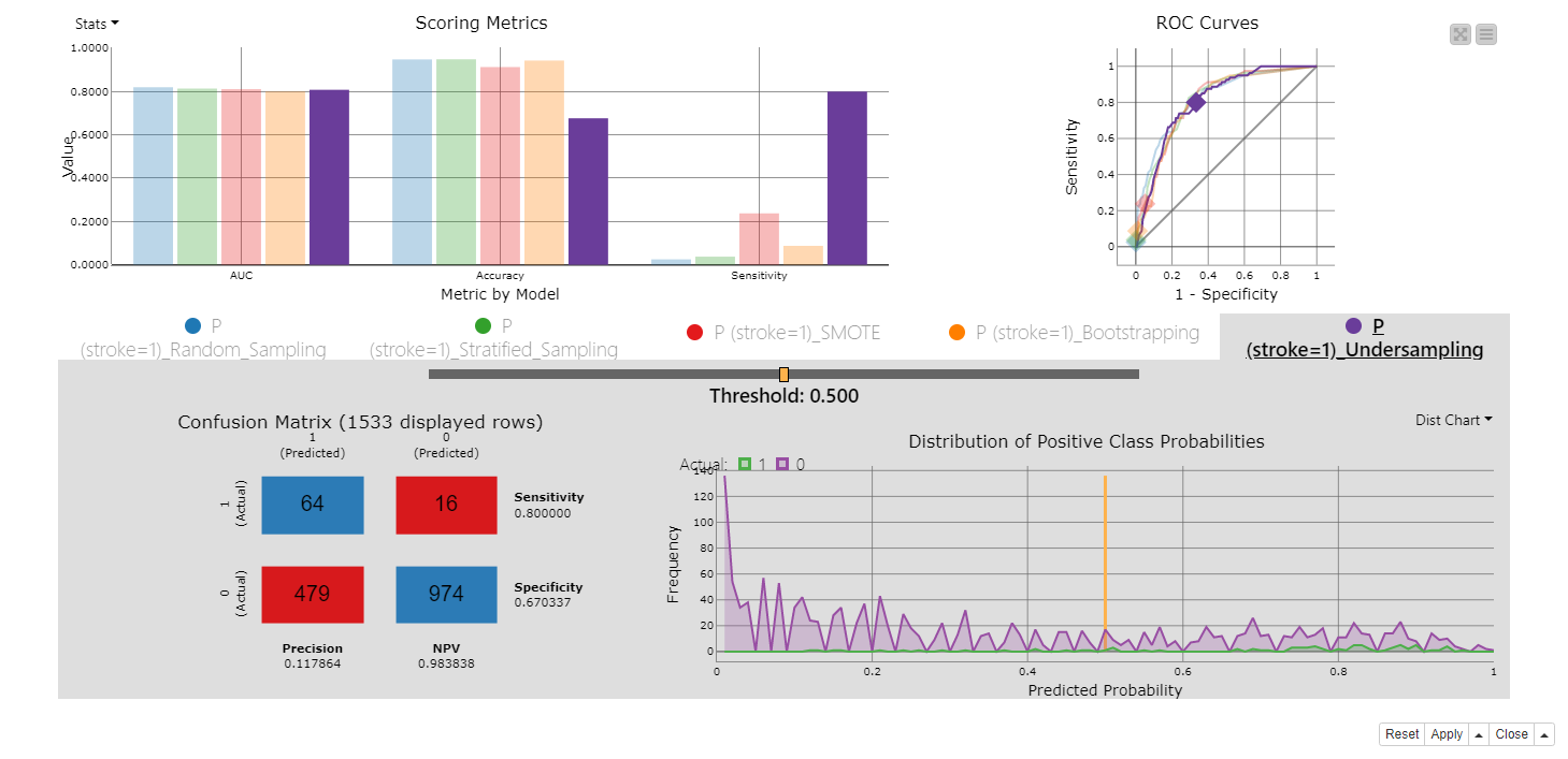
The top part of the view compares the models in terms of selected accuracy measures, such as area under the curve, overall accuracy, and sensitivity and also displays their ROC curves. You can see in the bar chart for the accuracy measures that if we do nothing to tackle class imbalance, that is using simple random partitioning (the blue bar) and stratified partitioning (the green bar) only, we obtain very similar - poor - results. In both cases, overall accuracy is almost 95% and the sensitivity is almost 0%. This means, the model is learning to classify only the majority class while having substantially no predictive ability for the minority class.
Instead, tackling class imbalance improves the model performance. In particular, using SMOTE on the training data (the red bar), we obtain an overall accuracy of 89% and a sensitivity score of 22%.
However, by far the best performing model is that the one where class imbalance was trained on undersampled training data (the purple bar), since it reaches a sensitivity value of 81%. If we take a closer look at the confusion matrix at the bottom part of the view, we can see that for 64 out of 75 individuals, stroke was correctly predicted. Although 479 individuals were mispredicted as patients who had a stroke when in fact they did not, in specific domains such as disease screening it is usually desirable to falsely alert healthy patients of a risk of suffering a stroke than missing a patient who is actually likely to suffer one.
Lessons Learned: The Choice of Sampling Technique Depends on the Data
Ultimately, the choice of sampling technique depends on the data and the problem you are trying to answer. Here we have illustrated several situations, explained the pros and cons of different sampling techniques, and highlighted how the sampling strategy can affect the accuracy of your model.
Download this workflow which we have built to try out and experiment with different strategies and review the results of each technique. Thank you for reading and happy data science-ing!
References
Illowsky, B., Dean, S. L., OpenStax College,, & Rice University,. (2013). Introductory Statistics