
Do you remember when we took you through the nine circles of hell with parameter optimization and a cup of tea? We introduced a parameter optimization workflow that uses four different machine learning models, individually optimizes the hyperparameters, and picks the best combination of machine learning method and hyperparameters for the user. However, the usual data scientist journey doesn’t end here. Having spent hours, days, or even (sleepless) nights exploring your data and finding the model with the best hyperparameters, you don’t want your model to be buried and forgotten somewhere on your computer. In real world situations, you would want to make your model predictions accessible to other people. Maybe even create a web application, where users could enter their data and get your model prediction with some helpful data visualizations.
In this blog post we will show you how to go from your trained model to a predictive web application with KNIME in three easy steps:
-
Model selection and parameter optimization
-
Integrated Deployment of the best performing model
-
Creating a web application
1. Model selection and parameter optimization
We took the Model Optimization and Selection workflow from the previous blog post as a starting point and did some adjustments.
This adjusted Model Optimization and Selection workflow (shown in Figure 1) is available for you to download from the KNIME Hub here.
Similar to the original workflow:
The adjusted workflow starts by reading data into the workflow. The dataset is a subset of 844 compounds, i.e. molecules, from a public data set available via https://chembl.gitbook.io/chembl-ntd/ (data set 19), which were tested for activity against CDPK1. Each compound is either “active” or “inactive”.
In contrast to the original workflow:
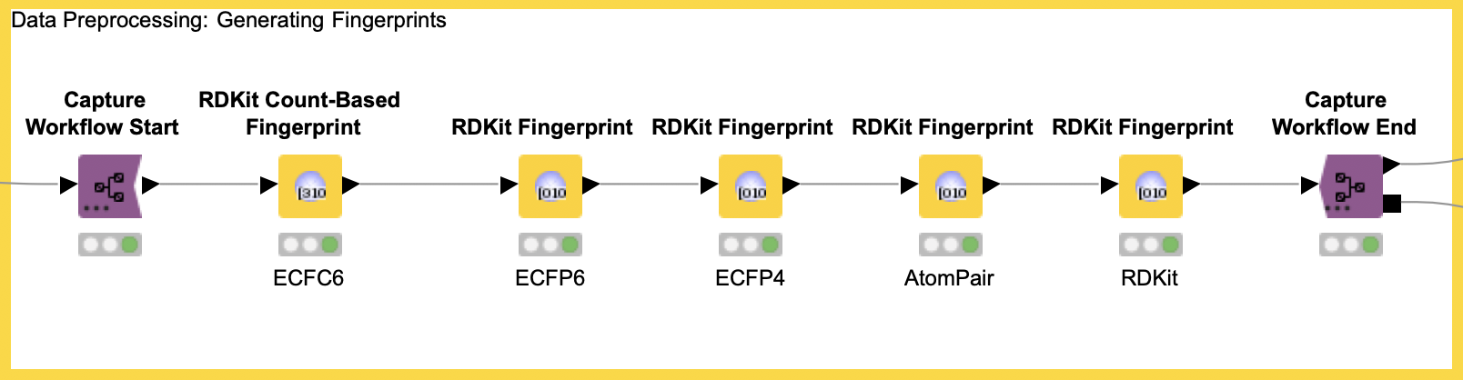
We integrate the data preprocessing in our adjusted workflow. In the “Generate Fingerprints” metanode, we compute five molecular fingerprints for the compounds using the RDKit nodes.
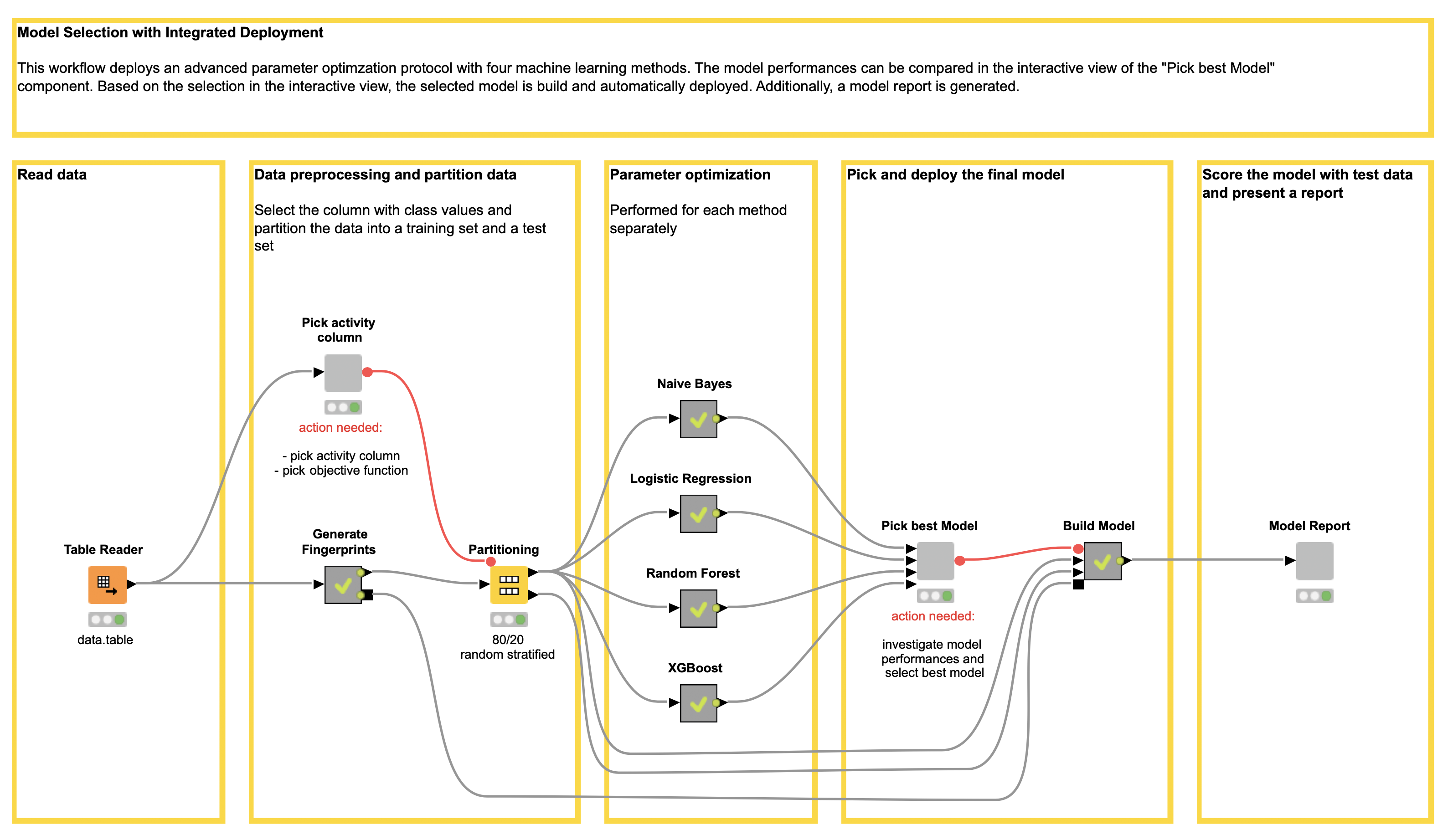
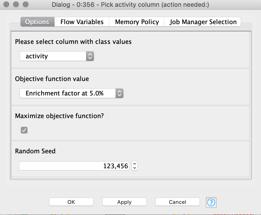
In the “Pick activity column” component the target column containing the class values (active, inactive) can be selected by the user (see Figure 2). Additionally, the user can select the objective function value. The objective function value is the value that will be optimized for each of the machine learning models. It is handy to define the objective function value beforehand in one place. This reduces the possibility of introducing mistakes by accidentally selecting different objective function values for each machine learning method. In our example, we choose an Enrichment Factor of 5% as the objective function value.
Based on our target column (i.e. activity), we perform a stratified partitioning of the data into a:
-
training set for parameter optimization and a
-
test set for scoring the best model.
Hyperparameter optimization
Similar to the original workflow, the hyperparameter optimization for each of the four machine learning methods is done in the corresponding metanodes: Naive Bayes, Logistic Regression, Random Forest and XGBoost. Please have a look at the previous blog post for a detailed description of the parameter optimization cycles.
Compare Model Performances
After optimizing each machine learning method, we want to compare the model performances and select the best model for our use case.
-
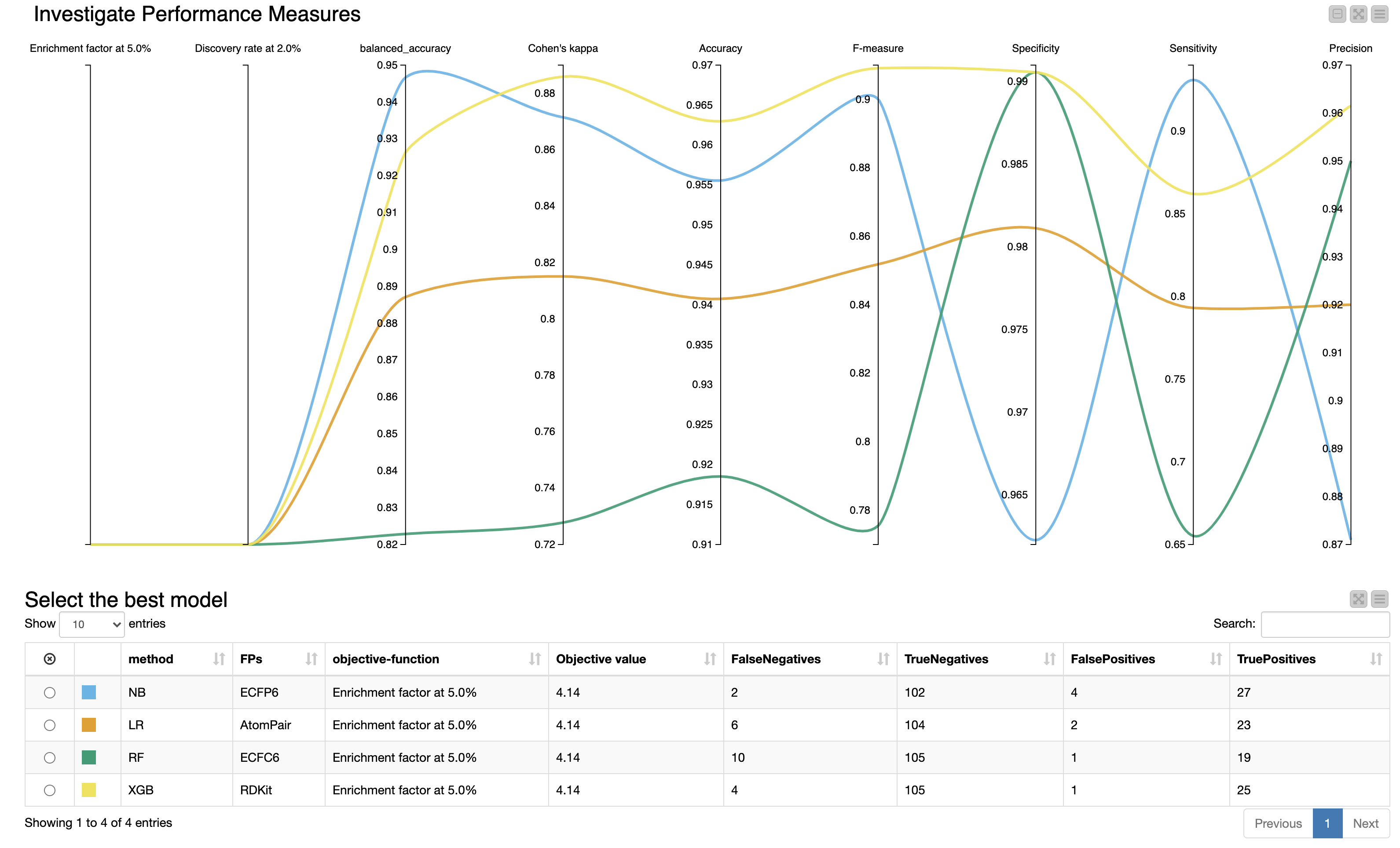
The “Pick best model” component provides an interactive view, which helps us evaluate the performance of each model (Figure 3).
-
The Parallel Coordinates Plot shows the values for the different model performance measures.
In our example, we optimized the models for the enrichment factor at 5% and all models perform equally well regarding both the enrichment factor at 5% as well as the discovery rate at 5%. Therefore, we have to take additional model performance measures into account. For our example, we will mainly focus on:
-
F-measure
-
Balanced accuracy
since those model performance measures are especially suited for imbalanced classes (as is the case for our dataset). For Cohen’s kappa and F-measure, the XGBoost model outperforms the other models. In terms of balanced accuracy, the XGBoost is the second best model. Therefore, we select the XGBoost model as the best model for our use case.
In the “Build model” component, the final model is trained and deployed (detailed description in the following section “Integrated Deployment”).
Report on Best Hyperparameter and Model Performance
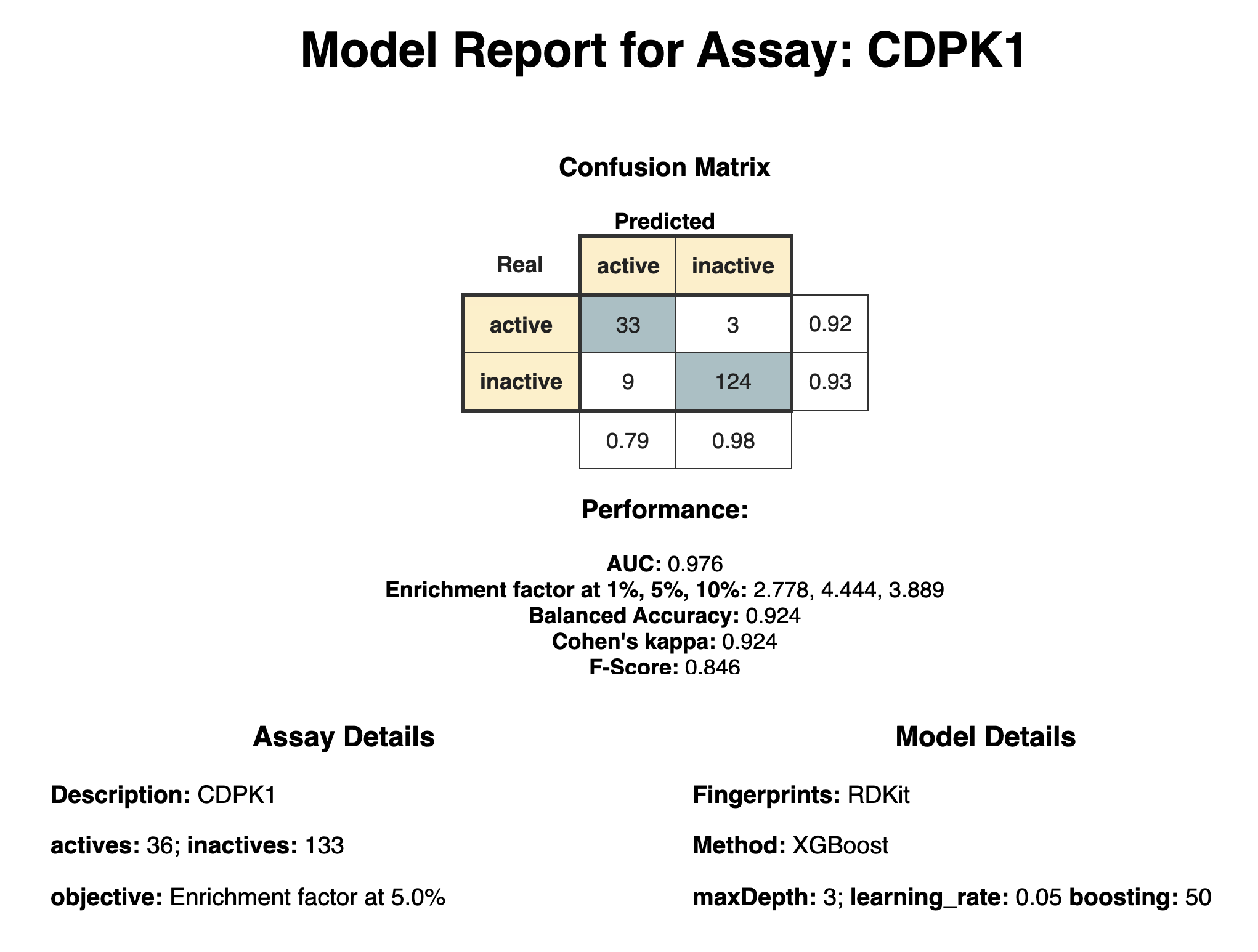
The last component, “Model Report”, creates a short report containing information about the best hyperparameter and performance of the model (see Figure 4). In our example, the XGBoost model using RDKit fingerprint was selected as it outperformed the other models in regards to Cohen’s Kappa.
2. Integrated deployment of the best performing model
To deploy your trained model, there are a few things that you need to keep in mind. The deployed workflow needs to include not only your trained model but also any data preprocessing that you did before training the model. Before KNIME Analytics Platform Version 4.2.0, that meant saving your trained model to a file and copying your preprocessing nodes to the deployed workflow, which increased the risk of mistakes.
Starting with KNIME Analytics Platform 4.2.0, there are some new nodes which can make your life much easier and help you to deploy your model in a more automated way (see this webpage on KNIME Integrated Deployment here). Now you can use the Capture Workflow Start and End nodes to define the workflow parts that you want to deploy. This means that the workflow parts that you captured will be written automatically to a separate workflow.
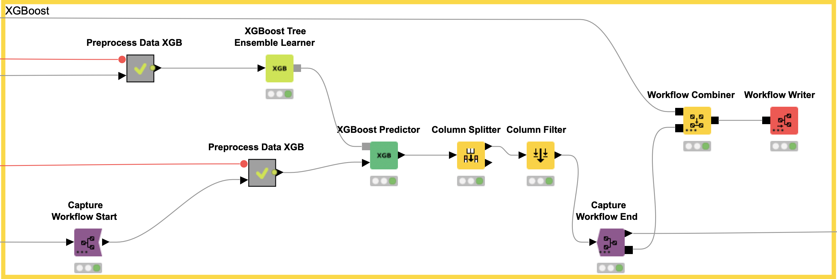
In our example, we capture the data preprocessing (e.g. computation of the five fingerprints) with the Capture Workflow Start and End nodes by simply inserting them at the beginning and end of our data preprocessing workflow, as shown in Figure 5. Similarly, model prediction is captured using the same nodes (see Figure 6). The Workflow Combiner node is used to join the two workflows. The red Workflow Writer node deploys the workflow automatically to the user-defined destination. That’s all you need to do.
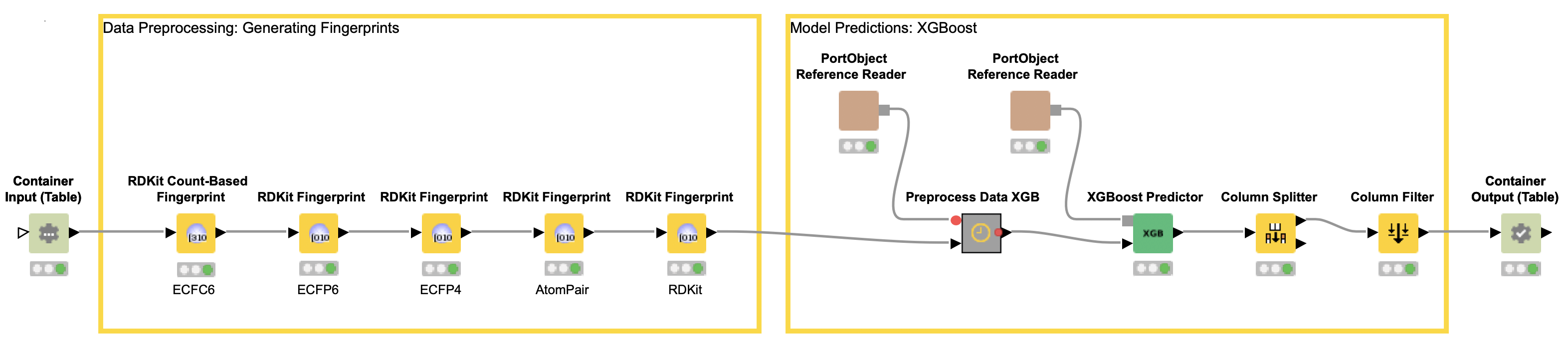
The deployed workflow is shown in Figure 7. The Container Input (Table) and Container Output (Table) nodes are added automatically. Those nodes enable the deployed workflow to receive a table from an external caller via a REST API and return the model prediction. At this point, we could deploy our model as a REST web service by simply copying the deployed workflow to a KNIME Server. This way, anyone could get predictions from our trained model using the KNIME Server REST API. However, most people do not use REST APIs but rather want a graphical interface where they can easily enter their data and get model predictions together with a useful visualization. So, let’s move on to the last step and create a small web application.
3. Creating a web application
To create a web application you need the KNIME Webportal which comes along with the commercial KNIME Server license. In case you are working with the open source KNIME Analytics Platform, you can still create and execute the web application workflow (see Figure 8) but you won’t be able to deploy the actual web application.
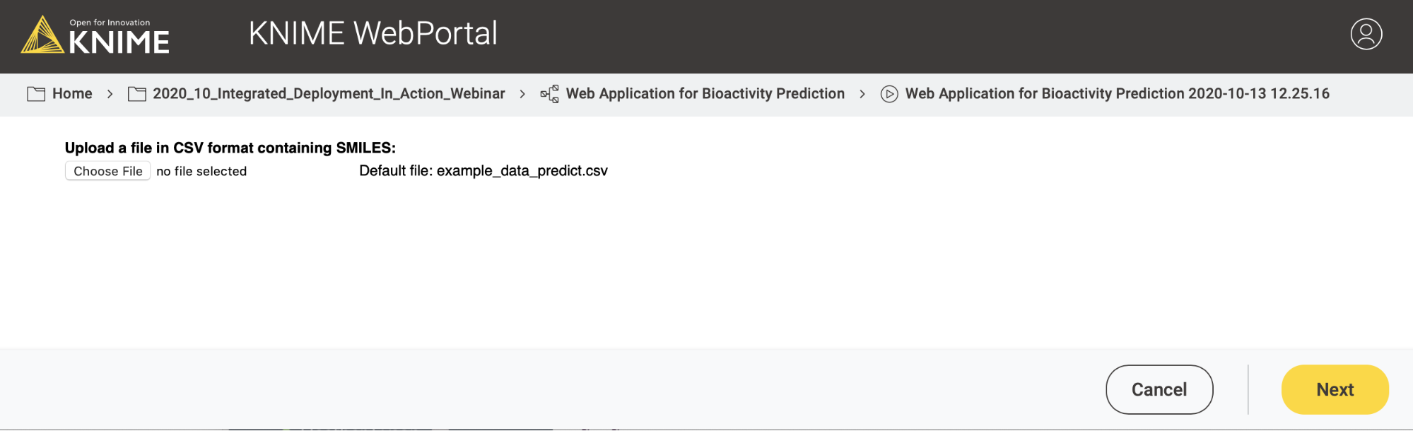
The workflow (shown in Figure 8) creates three views/user interactions points for our web application. The views are generated by components. The first component/view “File Input” (shown in Figure 9) enables the user to upload a file containing the compounds for which they want a model prediction (CDPK1 activity prediction).
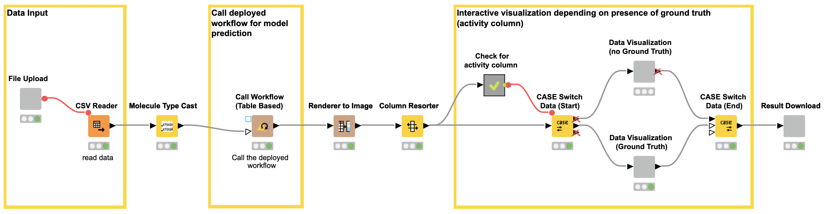
After the file upload, there are some nodes that process the input in the background and are not visible in the web application. For example, the Molecule Type Cast node converts the SMILES from a string format into a SMILES data format. The Call Workflow (Table Based) node passes the compounds to our deployed workflow (Figure 7). There the data is preprocessed (computing the molecular fingerprints) and the CDPK1 activity is predicted using the best performing model, in our case XGBoost. The predictions for each compound are returned as an additional column to our input table.
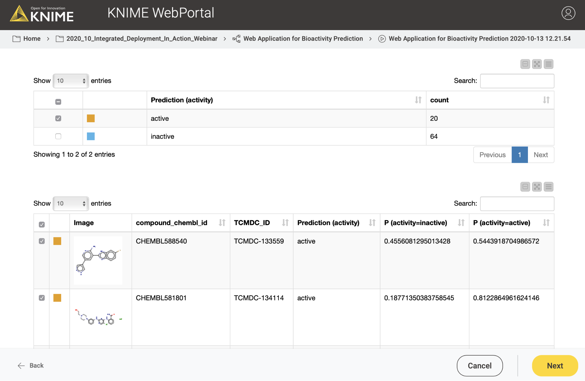
For the second view of the web application, we use a Case Switch node depending on the data that is uploaded by the user.
In the first case, the user uploads a data file which contains simply chemical structures, without any knowledge about its activity on CDPK1. The user simply wants a prediction for his/her data.
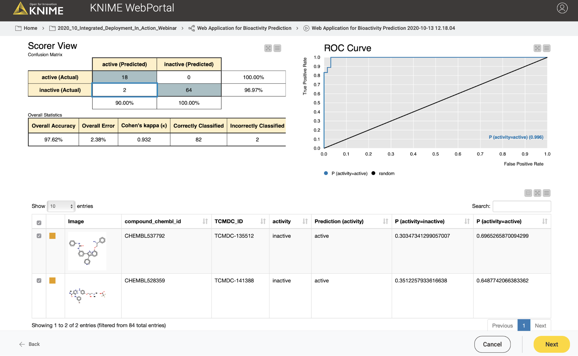
In the second case, the user might want to test or evaluate our model (some people like to do that). In that case, they will upload a file which, besides the chemical structures, also contains the true activity (“ground truth”) on CDPK1. If the activity column (“ground truth”) is available, we can also provide the confusion matrix and the ROC curve for the data (see Figure 10). So our workflow contains a metanode in which we determine if the activity column is available in the uploaded data file. Depending on the presence of the activity column, a different web application view is shown (Figure 10 vs Figure 11).
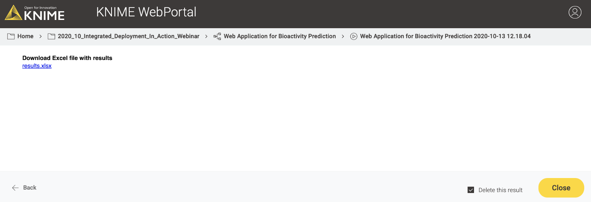
In the third and last view of the web application, the user can simply download the results of the model predictions including his/her selection in the interactive view as an Excel file (Figure 12).
Wrapping up
We showed you three simple steps to automatically get from training your machine learning model to building a predictive web application. You can adjust your parameter optimization and model selection pipeline by using the new integrated deployment nodes to automatically deploy the best model for your data. If you create a simple web application workflow for the KNIME Webportal you can easily make your trained model accessible to “consumers”.