
In a social networking era where a massive amount of unstructured data is generated every day, unsupervised topic modeling has became a very important task in the field of text mining. Topic modeling allows you to quickly summarize a set of documents to see which topics appear often; at that point, human input can be helpful to make sense of the topic content. As in any other unsupervised-learning approach, determining the optimal number of topics in a dataset is also a frequent problem in the topic modeling field.
In this blog post we will show a step-by-step example of how to determine the optimal number of topics using clustering and how to extract the topics from a collection of text documents, using the KNIME Text Processing extension.
You might have read one or more blog posts from the Will They Blend series. This blog post series discussed blending data from varied data sources. In this article today, we’re going to turn that idea on its head. We collected 190 documents from RSS feeds of news websites and blogs for one day (06.01.2017). We know that the documents are divided largely into two categories, sports and barbeques. In this blog post we want to separate the sports documents and barbeque documents by topic and determine which topics were most popular on that particular day. So, the question is will they unblend?
Note that the workflow associated with this post is available for download in the attachment section of this post, as well as on the KNIME Example Server.
Figure 1. Topic extraction workflow. You can download this workflow from the KNIME Hub here.
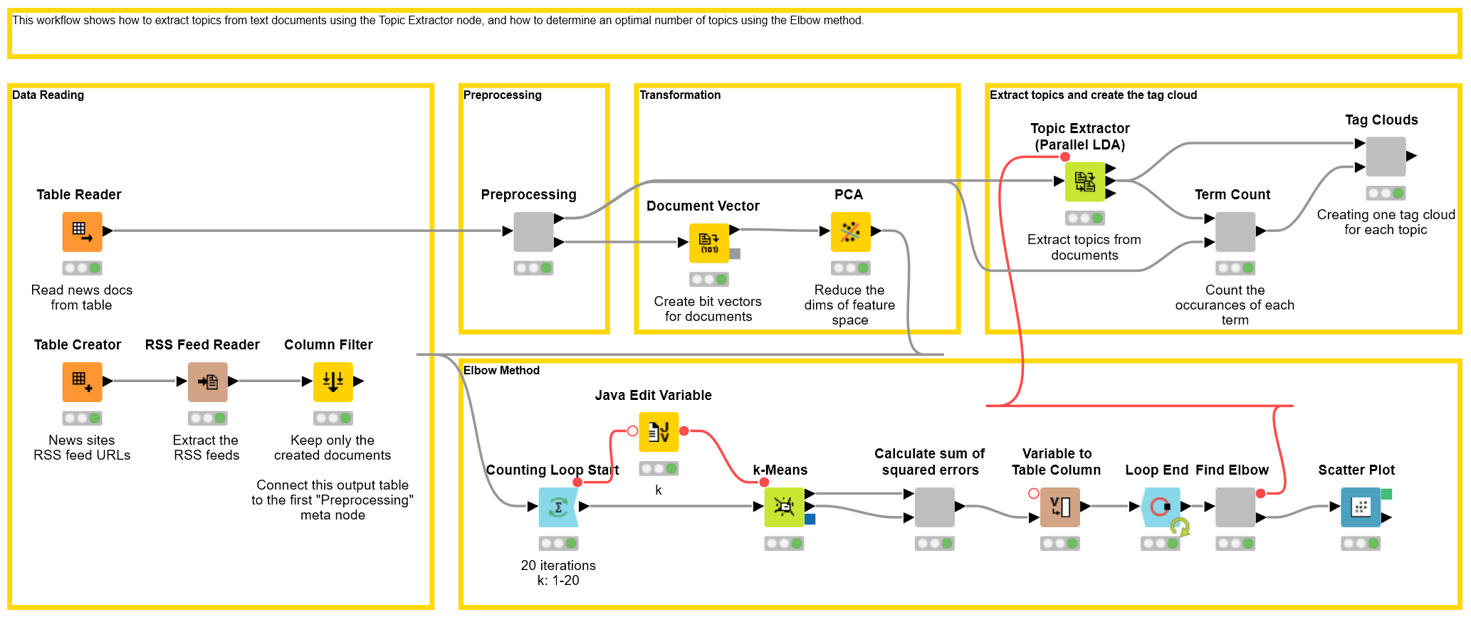
Reading Text Data
The first step starts with a "Table Reader" node, reading a table that already contains news texts from various news websites in text document format. An alternative would be to fetch the news directly from user-defined news websites by feeding their RSS URLs to the “RSS Feed Reader” node, which would then output the news text directly in text document format. The output of the "Table Reader" node is a data table with one column containing the document cells.
Figure 2. Reading textual data from file or from RSS News feeds.
Text Preprocessing I
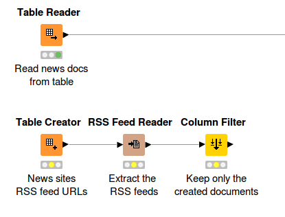
The raw data is subsequently preprocessed by various nodes provided by the KNIME Text Processing extension. All of the preprocessing steps are packed in the “Preprocessing” wrapped meta node.
First, all of the words in the documents are POS tagged using the “Stanford tagger” node. Then a “Stanford Lemmatizer”(*) is applied to extract the lemma of each word. After that, punctuation marks are removed by the "Punctuation Erasure" node; numbers and stop words are filtered, and all terms are converted to lowercase.
(*) A Lemmatizer has a similar function to a stemmer, which is to reduce words to their base form, however a lemmatizer goes further and uses morphological analysis to help remove the inflectional ending or plural form of a word and convert it to its base form, e.g the lemma of the word saw can be either see or saw depending on the position of the word in a sentence, and whether the word is a verb or a noun.
Figure 3. Basic text preprocessing: lemmatization, filtering of numbers, stop words etc. and case conversion.
Finding the optimal number of topics
Once the data have been cleaned and filtered, the “Topic Extractor” node can be applied to the documents. This node uses an implementation of the LDA (Latent Dirichlet Allocation) model, which requires the user to define the number of topics that should be extracted beforehand. It would be relatively easy if the user already knew how many topics they wanted to extract from the data. But oftentimes, especially in unstructured data such as text, it can be quite hard to estimate upfront how many topics there are .
There are a few methods you can choose from to determine what a good number of topics would be. In this workflow, we use the “Elbow” method to cluster the data and find the optimal number of clusters. It is o that the optimal number of clusters relates to a good number of topics.
Text Preprocessing II
Figure 4. Filtering of words based on frequency in corpus.
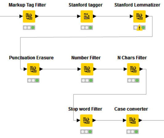
To use clustering, we need to preprocess the data again, this time by extracting the terms that we want to use as features for the document vectors. All of the preprocessing steps are packed into another wrapped meta node called “Preprocessing”. Basically the steps involve creating a bag of words (BoW) of the input data. It can be useful to remove terms that occur very rarely in the whole document collection as they don’t have a huge impact on the feature space, especially if the dimension of the BoW is very large. The document vectors are created next. For more details on how these steps are performed, please have a look at this post on Sentiment Analysis.
Note: After creating the document vectors, if the dimension of the feature space is still too large, it can be useful to apply PCA to reduce the dimensionality but keeping the loss of important information minimal.
The Elbow Method
Figure 5. Loop to compute k-means clusterings based in different values of k.
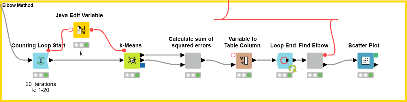
Now that we have converted our data into document vectors, we can start to cluster them using the “k-Means” node. The idea of the Elbow method is basically to run k-means clustering on input data for a range of values of the number of clusters k (e.g. from 1 to 20), and for each k value to subsequently calculate the within-cluster sum of squared errors (SSE), which is the sum of the distances of all data points to their respective cluster centers. Then, the SSE value for each k is plotted in a scatter chart. The best number of clusters is the number at which there is a drop in the SSE value, giving an angle in the plot.
Figure 6. Calculation of sum of squared errors for a clustering with a given k.
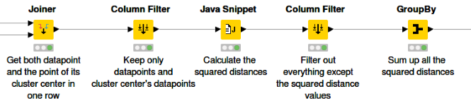
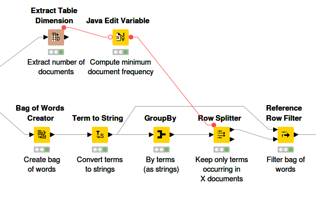
As we already mentioned, the “k-Means” node is applied to cluster the data into k clusters. The node has two output data ports: the first port contains a data table of all the document vectors and their correspondent cluster IDs to which they are assigned, and the second port contains vectors of all the cluster centers. Next, we use the “Joiner” node to join both output data tables based on their cluster IDs. The goal is to get both the document vectors and the vector of their respective cluster centers in each row so as to make the calculation easier. After that, the “Java Snippet” node is used to calculate the squared distance between a vector and its cluster center vector in each row. The SSE value for this certain k number of clusters is the sum of all the squared distances, where the sum is calculated by the “GroupBy” node.
In order to look for an elbow in a scatter chart this calculation is run over a range of numbers of k, which in our case is 1 to 20. We achieve this by using Loop nodes. The value k of the current iteration is provided as the flow variable and also controls the setting “k” of the k-Means node.
Figure 7. Plot of the sum of squared errors for all clusterings.
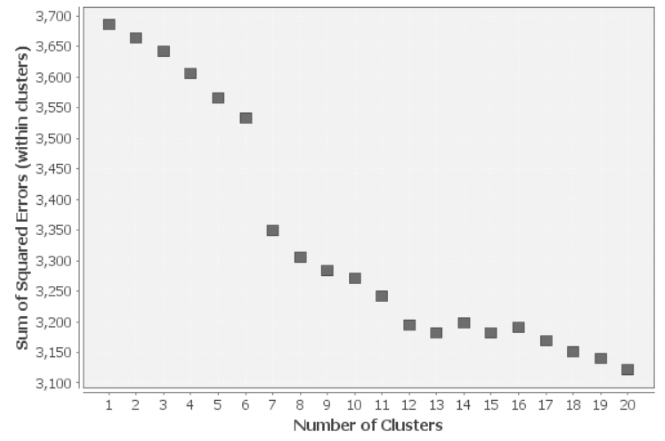
The “Scatter Plot” node is used to generate a scatter chart of the number of clusters k against the value of SSE. You will see that the error decreases as k gets larger. This makes sense because the more clusters there are, the smaller the distances between the data points and their cluster centers. The idea of the Elbow method is to choose the number of clusters at which the SSE decreases abruptly. This produces a so-called "elbow" in the graph. In the plot above you can see that the first drop is after k=6. Therefore, a choice of 7 clusters would appear to be the optimal number. The optimal number of clusters is determined automatically in the workflow, by taking the distances of subsequent SSE values and sorting the step with the largest distance on top. The related number k is then provided as the flow variable to the Topic Extractor node.
Note that the Elbow method is heuristic and might not always work for all data sets. If there is not a clear elbow to be found in the plot, try using a different approach, for example the Silhouette Coefficient.
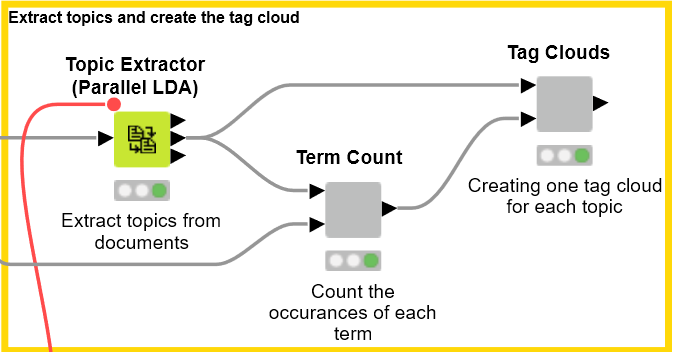
Extracting the Topics
Once we have determined the possible optimal number of topics for the documents, the Topic Extractor node can be executed. The node assigns a topic to each document and generates keywords for each topic (you can specify just how many keywords should be generated for each topic in the node dialog). The number of topics to extract is provided via a flow variable.
Figure 8. Topic extraction with the Topic Extractor node.
The extracted words for each topic are listed below:
- Topic 1: lions, tour, continue, zealand, world, round, player, cricket, gatland, england
- Topic 2: recipe, barbecue, bbq, chicken, lamb, kamado, pork, sauce, smoked, easy
- Topic 3: player, sport, tennis, court, margaret, derby, murray, mangan, world, declaration
- Topic 4: league, cup, manchester, club, season, united, city, goal, team, juventus
- Topic 5: bbq, sauce, recipe, turkey, brine, chicken, thanksgiving, breast, hunky, mad
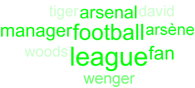
- Topic 6: football, wenger, league, arsène, manager, arsenal, woods, tiger, fan, david
- Topic 7: home, nba, cavaliers, lebron, final, james, los, golden, mets, team
Topic 1 is clearly about English sports. Topic 2 is about smoked bbq with chicken, lamb and pork. Topic 3 about tennis, Topics 4 and 6 about football (soccer). Topic 5 is again about bbq but focuses more on turkey and Thanksgiving. Topic 7 seems to be about American football. We have therefore found two topics about barbeques and five topics about sports.
We can now apply the “Tag Cloud” node to visualize the topics' most popular terms in an appealing manner. To do that, the keywords/terms generated by the “Topic Extractor” node have to be counted by their occurrences over the whole corpus. The steps are illustrated below.
Figure 9. Counting of extracted topic words in corpus.
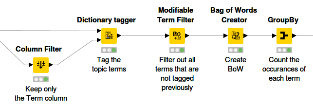
First of all, the “Dictionary Tagger” node is applied to tag only the topic terms. The goal is to filter out all terms that are not related to topics. This is done by using the “Modifiable Term Filter” node, which keeps those terms that have been tagged before and thus set to unmodifiable. After that, the BoW is created and the occurrences of each term are counted using the “GroupBy” node. Then for each topic a tag cloud is created, and the number of occurrences is reflected in the font size of each term.
The figures below shows the tag cloud for the topics English Sports, Thanksgiving barbeque, and football.
Figure 10. Tag cloud above showing topic English Sports.

Figure 11. Tag cloud above showing the Thanksgiving barbeque topic.
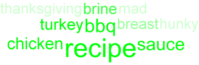
Figure 12. Tag cloud above showing the football topic.
It can be the case that the most popular terms are not really keywords, but rather some sort of stop words. To avoid this, the “IDF” node was used to calculate the IDF value for each term. All terms with low IDF values have been filtered out to make sure that only important terms will represent a particular topic.
The result of our workflow is satisfying as we have managed to cluster most of the data correctly and matched the extracted topics with the actual topics in the data.